1.  INTRODUCTION

A catchment's water yield is a fundamental problem in hydrology, referring to the volume of water available at the catchment outlet over a specified period of time. The yield is expressed for monthly, seasonal, or annual periods. Several approaches are available for the computation of water yield. These vary in complexity from simple empirical formulas to complex models based on continuous simulation. While the empirical formulas have limited applicability (Sutcliffe and Rangeley, 1960; Woodruff and Hewlett, 1970), the continuous simulation models require large amounts of data for their successful operation (Crawford and Linsley, 1966). A practical alternative is represented by conceptual models which use the water balance (or hydrologic budget) equation to separate precipitation into its various components (Hamon, 1963).

In this paper, we develop a conceptual model of annual water balance, suitable for application to a wide range of climatic conditions. The model separates annual precipitation into its three major components: surface runoff, baseflow, and vaporization. It is based on a two-step sequential application of a proportional relation linking two variables X and Y, such that the difference Z = X - Y asymptotically reaches an upper bound as X and Y grow unbounded. The generic form of the proportional relation has two parameters: λ, the initial abstraction coefficient, and Z_p, the potential value of Z = X - Y. Initial testing using L'vovich's (1979) catchment data shows that the model is applicable throughout a wide range of climatic settings.

2.  WATER BALANCE EQUATIONS

A water balance equation applicable to an individual storm is:

P = Q + L

(1)

in which P is precipitation, Q is surface runoff (also rainfall excess), and L is losses, or hydrologic abstractions (in millimeters, centimeters, or inches). The losses for an individual storm consist of interception, surface storage, and infiltration.

A water balance equation applicable on an annual basis is:

P = R + E

(2)

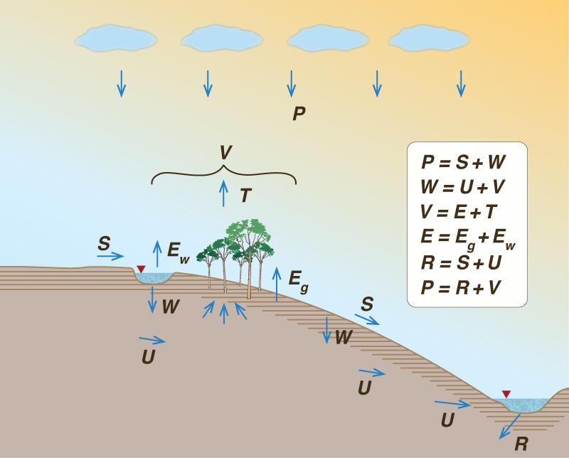
in which P is precipitation, R is runoff, including surface and subsurface runoff, and E is evapotranspiration (in millimeters, centimeters, or inches). In this equation, the term 'evapotranspiration' comprises all three types of evaporated moisture: (1) evaporation from vegetated surfaces, i.e. evapotranspiration, (2) evaporation from nonvegetated surfaces (bare ground), and (3) evaporation from water bodies.

Equations 1 and 2 are highly simplified models of a segment of the hydrologic cycle. For example, Eq. 1 does not describe the portion of surface storage that may eventually infiltrate into the ground. Likewise, Eq. 2 does not explicitly describe soil moisture, which is included in both runoff and evaporation. In fact, as shown by L'vovich (1979), a catchment's annual water balance is better described by a set of equations.

Annual precipitation P may be separated into two components (Fig. 1):

P = S + W

(3)

where S is surface runoff, i.e. the fraction of runoff originating on the land surface, and W is catchment welting, or simply 'wetting', the fraction of precipitation not contributing to surface runoff. (Note that Eq. 3 is the annual equivalent of Eq. 1.)

Fig. 1  Elements of the water balance.

Likewise, wetting consists of two components:

W = U + V

(4)

where U is baseflow, i.e. the fraction of wetting which exfiltrates as the dry-weather flow of rivers, and V is vaporization, the fraction of wetting returned to the atmosphere as water vapor (Lee, 1970). Deep percolation, i.e. the portion of wetting not contributing to either baseflow or vaporization, is a very small fraction of precipitation [a global average of less than 1.5%, according to L'vovich (1979)], and is neglected here on practical grounds.

Vaporization, which comprises all moisture returned to the atmosphere, has two components:

V = E + T

(5)

where E is nonproductive evaporation, hereafter referred to as 'evaporation', and T is productive evaporation, i.e. that resulting from plant transpiration, hereafter referred to as 'evapotranspiration.'

Evaporation has two components: (1) E_n, evaporation from nonvegetated areas of the Earth's surface and near-surface, i.e. from bare soil and small surface storage (puddles); (2) E_w, evaporation from sizable water bodies such as lakes, reservoirs, and rivers. Evapotranspiration is the evaporation from vegetated surfaces such as leaves and other parts of plants, a function of the physiological need of plants to pump moisture from the soil to maintain turgor and avail themselves of nutrients.

From Eqs. 3, 4, and 5, runoff consists of two components:

R = S + U

(6)

Likewise, precipitation P consists of two components:

P = R + V

(7)

Equation 7 is analogous to the well-known annual water balance Eq. 2. However, Eq. 7 is preferred here, because the term 'vaporization' clearly identifies the three sources of evaporated moisture (Eq. 5).

The set of Eqs. 3-7 constitute a set of water balance equations. Combining Eqs. 6 and 7 leads to:

P = S + U + V

(8)

that is, annual precipitation is separated into its three major components: surface runoff, baseflow, and vaporization. Significantly, Eq. 8 assumes that the change in soil-moisture storage from year to year is negligible, an assumption which is useful as a first approximation.

Equations 4 and 7 allow the definition of water balance coefficients. The baseflow coefficient is (L'vovich, 1979):

U            U Ku = ____ = ________          W        U + V

(9)

and the runoff coefficient is:

R           R Kr = ____ = ________          P         R + V

(10)

These coefficients vary as a function of prevailing climate, theoretically within the range 0-1. The prevailing climate is characterized by global wind circulation, mean latitude and altitude, aspect, geomorphology, proximity to the ocean, type of vegetation, and land use. In arid and semiarid regions, the water balance coefficients are low, typically less than 0.2, and may approach zero in hyperarid cases. In humid tropical regions, the coefficients are high, often greater than 0.5, with the runoff coefficient K_r approaching unity in some unusual cases of extreme humidity (L'vovich, 1979). However, there are exceptions such as a swamp or marsh (wetland), where K_r is typically a low value because of the increased evapotranspiration potential.

3.  THE CONCEPTUAL MODEL

A significant feature of the water balance equations (Eqs. 3-7) is that they all have the same structure, in which a quantity X is expressed as the sum of two components Y and Z:

X = Y + Z

(11)

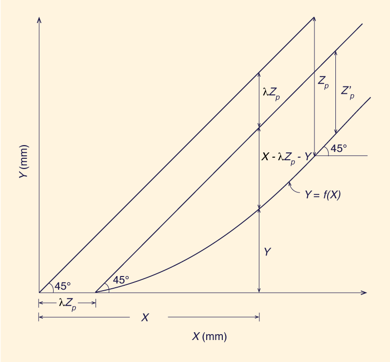
L'vovich (1979) has shown that Eq. 3 can be modeled by a proportional relation such that wetting asymptotically reaches an upper bound (W → W_p) as precipitation and surface runoff increase unbounded (P → ∞; S → ∞). It is noted that a similar relation is the basis of the SCS runoff curve number model, which solves Eq. 1 (US Department of Agriculture Soil Conservation Service (USDA SCS), 1985). L'vovich (1979) has also shown that Eq. 4 can be modeled by the same type of relation, i.e. one where vaporization reaches an upper bound asymptotically (V → V_p) as wetting and baseflow increase unbounded (W → ∞; U → ∞). In this way, the sequential two-step separation of annual precipitation into its three major components, surface runoff, baseflow, and vaporization, is accomplished.

The generic form of the proportional relation is, according to the SCS model (USDA SCS, 1985),

X - λ' Zp' - Y              Y _______________ = ____________           Zp'                X - λ' Zp'

(12)

in which Y = f(X) and λ' is the initial abstraction coefficient. The initial abstraction is I_a = λ' Z_p', in which Z_p' is the potential value of Z', i.e. an upper bound to Z' = X - λ' Z_p' - Y.

In this paper, the initial abstraction is alternatively defined as I_a = λ Z_p in which Z_p is the potential value of Z = X - Y (Fig. 2). This leads to a slightly modified form of the proportional relation:

X - λ Zp - Y               Y _______________ = ____________       (1 - λ)Zp             X - λ Zp

(13)

Fig. 2  Definition sketch for initial abstraction coefficient λ and potential Zp.

Equation 13 has a significant advantage over Eq. 12. Unlike λ', which has no theoretical upper bound, λ is limited in the range 0 ≤ λ ≤ 1. The initial abstraction coefficient λ is dimensionless; the units of Z_p are those of X and Y (millimeters, centimeters, or inches).

For the special case of zero initial abstraction (λ = 0), Eq. 13 reduces to:

X - Y          Y _________ = ____       Zp           X

(14)

Solving Eq. 13 for Y = f(X) leads to:

(X - λ Zp)2 Y = __________________           X + (1 - 2λ) Zp

(15)

subject to X > λ Z_p; Y = 0 otherwise.

Using Eq. 15, the surface runoff submodel is:

(P - λs Wp)2 S = ____________________           P + (1 - 2λs) Wp

(16)

subject to P > λ_sW_p, and S = 0 otherwise, where λ_s is the surface-runoff initial abstraction coefficient. From Eq. 3,

W = P - S

(17)

Likewise, the baseflow submodel is:

(W - λu Vp)2 U = ____________________           W + (1 - 2λu) Vp

(18)

subject to W > λ_u V_p, and U = 0 otherwise, where λ_u is the baseflow initial abstraction coefficient. From Eq. 4,

V = W - U

(19)

Thus, given annual precipitation and a set of initial abstraction coefficients λ_s and λ_u and potentials W_p and V_p, Eqs. 16-19 are used to separate annual precipitation into surface runoff, baseflow, and vaporization. Then, runoff is calculated by Eq. 6, and the baseflow and runoff coefficients K_u and K_r are calculated using Eqs. 9 and 10, respectively.

4.  MODEL CALIBRATION

In the absence of data, the initial abstraction coefficients and potentials are estimated from past experience in similar climatic settings. When data are available, the model parameters can be calibrated. For λ = 0, Z_p is solved from Eq. 14:

X (X - Y) Zp = ___________               Y

(20)

For λ > 0, Z_p is solved from Eq. 13:

X + [1/(2λ)] {(1 - 2λ) Y - [(1 - 2λ)2 Y 2 + 4λ (1 - λ) X Y]1/2} Zp = ________________________________________________________                                                   λ

(21)

To calibrate the model parameters based on X-Y data, the following recursive procedure is suggested:

1. Set λ = 0 and Δλ = 0.01.

2. Use Eq. 20 or Eq. 21 to calculate a Z_p for each X - Y pair, i.e. a Z_p array.

3. Calculate the mean, standard deviation, and coefficient of variation of the Z_p array.

4. Stop when the coefficient of variation of the Z_p array has reached a minimum. Otherwise, increase λ by Δλ and go back to Step 2.

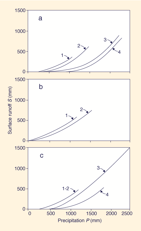
The calibrated λ is that for which the coefficient of variation of the Z_p array is a minimum. The calibrated Z_p is the mean of the Z_p array corresponding to the calibrated λ.

This procedure was applied to L'vovich's catchment data (1979), and the results of the calibration are shown in Tables 1 and 2. On the basis of this initial application, a tentative classification of parameter ranges is suggested: initial abstraction coefficient λ (dimensionless): low (0 < λ ≤ 0.1), average (0.1 < λ ≤ 0.3), high (0.3 < λ ≤ 0.5), and very high (0.5 < λ ≤ 1); potential Z_p (mm): low (0 ≤ Z_p ≤ 1000), average (1000 < Z_p ≤ 3000), high (3000 < Z_p ≤ 5000), and very high (Z_p > 5000).

Table 1 shows calibrated values of surface-runoff initial abstraction coefficient λ_s and wetting potential W_p for nine P - S data sets included by L'vovich (1979) (Fig. 3). Analysis of Table 1 leads to the following conclusions:

1. Arctic-subarctic plains and subarctic forests in Canada have λ_s, = 0, and low to average W_p (889-1578 mm). The nearly frozen ground produces an immediate surface runoff response, in relation to the amount of precipitation.

2. Mountain conifer forests in Africa, and mountain meadows, steppes, and savannas in South America have low λ_s (0.02-0.06), and average W_p (1789-2164 mm).

3. Savannas in Africa and South America have average λ_s (0.18-0.22), and average (bordering on high) W_p (2627-2944 mm).

4. Evergreen sclerophyll forests and scrub in Africa, and wet evergreen forests in the mountains of South America have average to high λ_s (0.23-0.31), and average W_p (1326-1517 mm).

5. Humid evergreen forests in Africa have very high λ_s (0.54) and average W_p (1970 mm). The very high initial abstraction produces a sluggish surface runoff response.

Fig. 3  Precipitation-surface runoff relations for selected biogeographical regions in (a) Africa, (b) Canada, and (c) South America (See Table 1 for explanation of curve numbers).

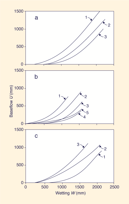
Table 2 shows calibrated values of baseflow initial abstraction coefficient λ_u and vaporization potential V_p for 11 W - U data sets included by L'vovich (1979) (Fig. 4). Analysis of this table leads to the following conclusions:

1. Southeastern wet forests in North America have λ_u = 0 and very high V_p (6110 mm). This produces an immediate baseflow response, in relation to the amount of wetting. However, this is tempered by the very high value of vaporization potential.

2. Subarctic forests and temperate steppes in North America have low λ_u (0.09-0.10), whereas V_p is low for the subarctic forests (796 mm) and high for temperate steppes (4246 mm).

3. Mixed forests with moderate continental climate in North America and wet evergreen forests in the mountains of South America have low to average λ_u (0.10-0.13) and average V_p (1294-1856 mm).

4. Plains and wooded steppes in North America and high mountain meadows in South America have average λ_u (0.19-0.25), whereas V_p is low for high mountain meadows (977 mm) and average for plains and wooded steppes (2047 mm).

5. Mountain conifer forests, evergreen sclerophyll forests and scrub, and mountain landscapes in Africa, and savannas in South America have high λ_u (0.35-0.48), with low to average V_p (903-1797 mm).

Fig. 4  Wetting-baseflow relations for selected biogeographical regions in (a) Africa, (b) Canada, and (c) South America. (See Table 2 for explanation of curve numbers).

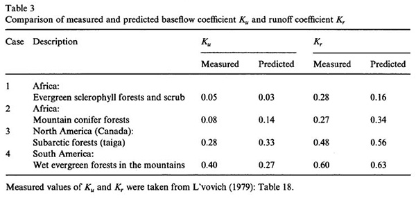
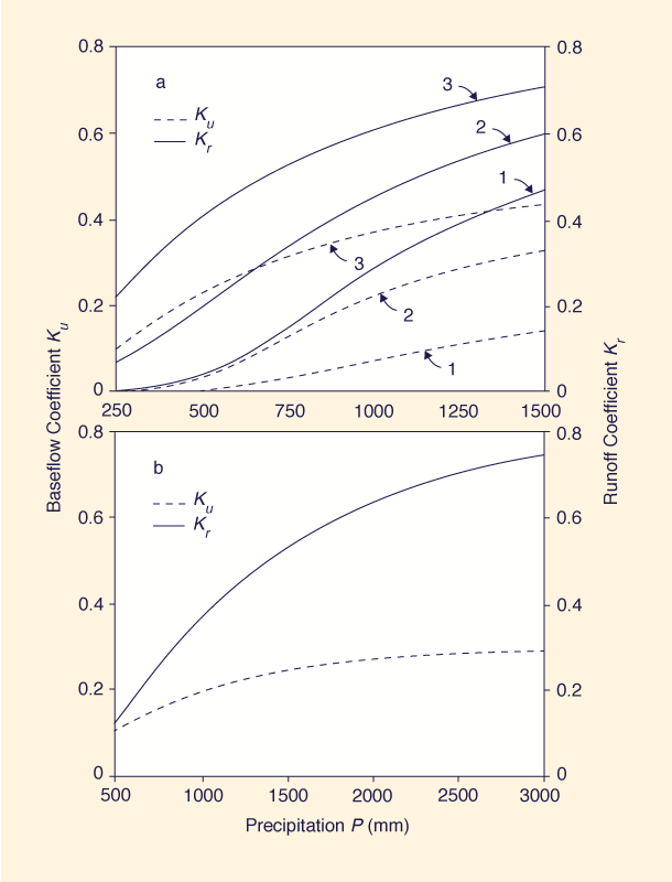
Table 3 shows a comparison of baseflow and runoff coefficients reported by L'vovich (1979) and predicted by the conceptual model developed herein. It is seen that the conceptual model is reasonably predictive for a wide range of climatic conditions. Figure 5 shows calculated baseflow and runoff coefficients for selected biogeographical-climatic regions shown in Table 3. It is seen that the coefficients predicted by the conceptual model are responsive to variations in precipitation input.

Fig. 5  Baseflow and runoff coefficients as a function of mean annual precipitation: (a) Cases 1, 2, and 3; (b) Case 4. (See Table 3 for explanation of curve numbers).

The wetting potential W_p is an upper bound to the fraction of annual precipitation that can be retained by a given catchment. A typical catchment is likely to feature several areas, each with a wetting potential W_pi covering a partial area A_i. A wetting potential spatially weighted for the entire catchment is:

∑ (Wpi Ai ) Wp = ___________               ∑ Ai

(22)

The vaporization potential V_p is an upper bound to the fraction of annual wetting that can evaporate from a given catchment. A typical catchment is likely to have three distinct types of surfaces: (1) vegetated surfaces, with an evapotranspiration potential T_pv covering a partial area A_v; (2) nonvegetated surfaces, with an evaporation potential E_pn covering a partial area A_n; (3) free-water surfaces, with an evaporation potential E_pw covering a partial area A_w. A vaporization potential spatially weighted for the entire catchment is:

Tpv Av + Epn An + Epw Aw Vp = ___________________________                      Av + An + Aw

(23)

5.  SUMMARY

A conceptual model of a catchment's water balance is formulated. The model is based on the sequential separation of annual precipitation into surface runoff and wetting, and wetting into baseflow and vaporization. The separation is based on a proportional relation linking the three variables involved at each step. The generic form of the proportional relation is (X - λZ_p - Y)/[(1 - λ) Z_p] = Y/(X - λZ_p), in which X is the independent variable, Y is the dependent variable, λ is the initial abstraction coefficient, and Z_p is the potential value of the difference Z = X - Y.

Given a set of model parameters, the model can separate annual precipitation into its three major components: surface runoff, baseflow, and vaporization. Furthermore, baseflow and runoff coefficients are characterized as a function of climate. The model can be used for estimates of annual water yield throughout the climatic spectrum. An initial application of the model to L'vovich's (1979) catchment data provided encouragjng results. Additional research is needed to determine initial abstraction coefficients and potentials for a wide range of associated biogeographical regions and climatic settings.

ACKNOWLEDGMENTS

The present study was performed in Spring 1994, while A.V. Shetty was at San Diego State University, on leave from the Hard Rock Regional Centre, National Institute of Hydrology, Belgaum, Karnataka, India. His leave was funded by the United Nations Development Programme.

REFERENCES

Crawford, N. H. and R. K. Linsley. 1966. Digital simulation in hydrology: the Stanford watershed model IV. Stanford Univ. Dep. Civ. Eng. Tech. Rep. 39.

Hamon, W.R. 1963. Computation of direct runoff amounts from storm rainfall. Int. Assoc. Sci. Hydrol. Publ., 63: 52-62.

Lee, R. 1970. Theoretical estimates versus forest venter yield. Water Resour. Res., 6(5): 1327-1334.

L'vovich, M. I. 1979. World water resources and their future. Original in Russian. English translation, American Geophysical Union, Washington, DC.

Sutcliffe, J. V. and W. R. Rangeley. 1960. Variability of annual river flow related to rainfall records. Int. Assoc. Sci. Hydrol. Publ., 76: 182-192.

U.S. Department of Agriculture Soil Conservation Service (USDA SCS). 1985. National Engineering Handbook, Section 4: Hydrology. SCS, Washington, DC.

Woodruff, J. F. and J. D. Hewlett. 1970. Predicting and mapping the average hydrologic response for the Eastern United States. Water Resour. Res., 6(5): 1312-1326.