1. INTRODUCTION The simplified methods of channel routing enjoy a position of preeminence within the gamut of available routing methods. These methods are simple to formulate and use, and may well account for most of the flood wave phenomena when practical applications are considered. The more refined versions simulate the diffusion wave model; therein lies their inherent strength.
A simplified method which is receiving increased attention is a Muskingum method in which the routing parameters are calculated based on channel and grid characteristics (1), herein referred to as Muskingum diffusion model. Its numerical behavior, however, is not completely understood. A direct consequence of insufficient spatial resolution is the notorious negative outflows which have been documented in certain cases (3,10). Until the reason for this anomaly is identified, the simplified methods will suffer from a lack of credibility. This can only hamper their wide acceptance for practical channel routing applications. The objective of this paper is, thus, twofold: (1) To review and examine recent contributions regarding spatial and temporal resolution in Muskingum diffusion models; and (2) to develop a criterion for spatial resolution to preserve the acccuracy of the method. Accuracy here is understood to mean that which is attainable within the framework of diffusion wave routing. 2. RECENT CONTRIBUTIONS ON ACCURACY CRITERIA
Koussis (2) was among the first to recognize the effect of insufficient spatial resolution on the hydrograph calculated by the Muskingum diffusion model, and to tie this effect to the grid size.
in which Δt = time step; Δx = space step; X = Muskingum parameter; and c = flood wave celerity for the reference flow. Koussis did not elaborate on how Eq. 1 was developed, and it is attributed here to his experience with the method. In their recent review of approximate flood routing methods, Weinman and Laurenson (10) focus on the Muskingum diffusion model and its variations. They point out the possibility of unrealistic negative outflows, but suggest that for practical purposes these negative outflows are small enough and sufficiently short-lived to be ignored if the following inequality is satisfied:
in which Tr = period-of-rise of the inflow hydrograph. The striking similarity between Koussis' and Weinman and Laurenson's criteria is apparent. A basis for comparison can be implemented if Tr is expressed in terms of Δt. Assuming that in a given case Tr / Δt = n is an integer greater than 5, Eq. 2 reduces to:
which indicates that Koussis' criterion is more conservative in the estimation of Δx than Weinmann and Laurenson's. The writers elsewhere (7) reported the results of preliminary findings that seemed to indicate that if accuracy is to be preserved (i.e., avoidance of negative outflows), the following inequality should hold:
in which C and D are Courant and cell Reynolds numbers, respectively, defined as follows:
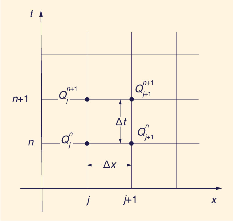
in which qo = reference unit-width discharge; and So = equilibrium water surface slope. Ponce and Theurer further stated that a value of ξ = 0.25 provided satisfatory accuracy in most cases. Kundzewicz (3) has applied the convolution method of analysis to the Muskingum diffusion model, and concluded that Eq. 2 does not hold for the general case. He further stated that a search for a general condition to supress negative outflows may prove to be fruitless. 3. CHOICE OF SPACE AND TIME STEPS Accuracy criteria such as Eqs. 1, 2 or 4 provide guidelines for the selection of space and time steps if negative outflows are to be eliminated. Following Ponce and Yevjevich (5), space and time steps are used together with channel and flood wave descriptors to calculate the routing parameters C and D, Eqs. 5 and 6. In turn, these parameters are used in the routing equation (Fig. 1):
in which C1, C2 and C3 are defined as follows:
Choice of space step. Given Eqs. 1, 2 and 4, the choice of space step is not altogether clear.
However, this condition suffers from a significant drawback; it is undefined for X = 0. In Muskingum diffusion routing, X = 0 implies that Δx is fixed, and Eq. 11 could no longer be applicable. The same type of criticism holds for Eq. 2. Equation 4, on the other hand, is expressed in terms of D rather than X, and an expression for the upper limit on Δx based on this equation is:
The question of a lower limit on Δx is also one that has led to some confusion, primarily due to the existence of a functional relationship between X and Δx:
Historically, the parameter X has been interpreted as a weighting factor, and this led Miller and Cunge (4), among others, to suggest a lower bound for X: X ≥ 0. This is echoed in Weinmann and Laurenson's review (10), which states (p. 1529): "Since X may not realistically decrease below zero, there is a limit to the allowable degree of subdivision, which implies a lower limit on Δx." Given
The right-hand side of Eq. 14 is immediately recognized as the "characteristic reach length" first identified by Kalinin and Milyukov (4) in connection with the routing method bearing their name.
Further analysis and experience with the method has shown, however, that in fact there is
no theoretical lower limit on Δx. Ponce and Theurer (7), as well as others (3,9),
have reported experience with Δx values violating Eq. 14, and yet with no physical unreality whatoever attached to the results of the computations. The reason for this behavior is apparent when the moment-matching characteristic of Eq. 13 is recognized. As long as this equation is satisfied, Δx may be arbitrarily chosen to violate Eq. 14, implying the possibility of negative values of X.
Choice of Time Step. The criterion for selecting the time step has also led to some confusion.
in which n = an integer having a minimum value of 5. In practice, hydrographs are skewed to the right; therefore, Eq. 15 guarantees a satisfactory level of temporal resolution. In addition to the previously given requirement of temporal resolution, there is a question as to whether the Muskingum diffusion model is bound by the Courant numerical stability criterion usually applicable to hyperbolic problems. If this is the case, then an additional constraint on Δt should be imposed:
which follows from:
Practical computations, however, have shown that violating Eqs. 16 and 17 does not lead to numerical instability. This behavior is explained by recalling that the method is essentially a finite difference formulation of the kinematic wave equation. In theory (6), this feature provides unconditional stability with respect to the Courant condition, thereby invalidating Eq. 17. A lower limit on Δt is mainly a question of computational resources. A decision on this matter is left to the individual modeler. Accuracy Criteria. From the preceding analysis, it follows that there is no theoretical justification for a lower limit on either Δt or Δx. Furthermore, while there is an upper limit on Δt given by the temporal resolution requirement, a similar upper limit on Δx is not clearly discernible. Given Eqs. 5, 6 and 13, Koussis' criterion is modified here and expressed in terms of C and D:
In this form, the overdeterminacy of Eq. 11 is removed. In effect, fo X = 0, D = 1 and Eq. 18 reduces to C ≥ 0. Since X = 0 implies that Δx is finite (Eq. 6), the condition C ≥ 0 reduced to the trivial one Weinmann and Laurenson's criterion, Eq. 3, leads to
and similar comments to that of Koussis' apply. Ponce and Theurer's remains:
The following section describes a program of numerical experiments designed to throw additional light onto the question of accuracy criteria. Consistency. Closely related to accuracy is the subject of consistency of a simplified routing method such as the one treated here. In the context of this study, accuracy refers to the avoidance of physically unrealistic negative outflows; consistency refers to the abiliity of the routing method to produce the same results regardless of grid size. For instance, if a certain hydrograph is obtained at the end of a given channel reach using ten (10) space steps, a consistent method would produce the same hydrograph if instead only two (2) space steps had been used. Consistency, as previously defined, is to be used within the framework of a simplified routing method in which the objective is to optimize the numerical diffusion by making it match the physical diffusion. This concept should not be confused with the property of consistency of a conventional finite difference scheme, in which the objective is to minimize the amount of numerical error in order to properly solve the differential equation under consideration. 4. NUMERICAL EXPERIMENTS A program of numerical experiments was carried out in order to evaluate the accuracy (and therefore, consistency) of the Muskingum diffusion routing described by Eqs. 7-10. The following considerations were used in the design of the program:
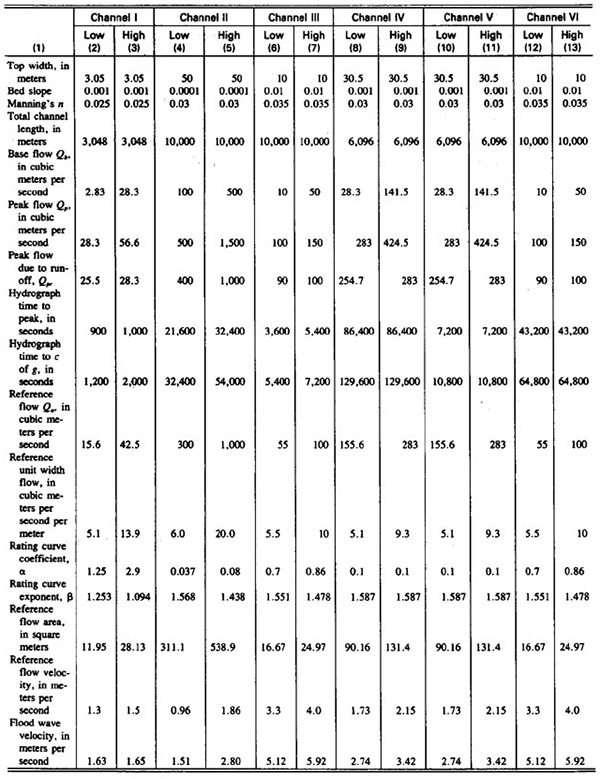
Six hypothetical channels were developed and tested in the course of this study. For each channel, two flow conditions were specified: (1) A low base flow; and (2) a high base flow. Each channel and flow condition was tested by routing the same hydrograph through 12 different grid specifications, making a total of 144 runs. The 12 grid specifications represented combinations of three (3) time steps and four (4) space steps. To simulate natural hydrographs, a gamma distribution was used as the inflow hydrograph. This function is of the following form:
in which Qt = inflow at time t; Qb = base flow; Qp = peak flow; tp = time from beginning of direct runoff to peak of hydrograph; tg = time from beginning of direct runoff to center of gravity of hydrograph; and m is given by the following equation:
Table 1 shows channel and hydrograph characteristics for the twelve (12) testing series. A detailed summary of the results of the numerical experiments is given in Ref. 8.
5. ANALYSIS OF RESULTS
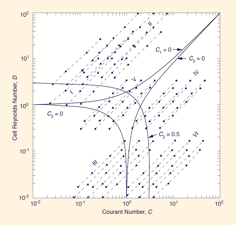
The results of the numerical experiments can be interpreted in the light of the two routing parameters: Courant number, C, and cell Reynolds number, D. To start with, it is noted that Δx is inversely proportional to both C and D. Therefore, the larger the Δx, the smaller the values of Figure 2 is a logarithmic plot of the values of C and D associated with all runs in the testing program. Also shown in this figure are the lines for C1 = 0, C2 = 0, and C3 = 0. An analysis of the numerical results strongly indicates that accuracy is dependent on the value of C2. Negative values of C2 are invariably associated with dips in the rising portion of the outflow hydrograph, indicating the tendency of outflows to become "negative" (i.e., values less than the base flow). This tendency increases as the value of C2 increases in the negative range.
Values of C2 in the range 0.0-0.5 do not show dips in the outflow hydrograph. However, depending on the problem, small inaccuracies in the calculated hydrographs may still remain. >
Values of C2 in excess of 0.5 are associated with hydrographs which do not show any of the previous anomalies. In addition, once accuracy is achieved, say for C2 ≥ 0.5, consistency follows.
6. SPATIAL RESOLUTION ACCURACY CRITERIA The experimental evidence suggests that C2 and only C2 is determinant of accuracy. In fact, values of C1 and C3 were monitored throughout the testing series, and negative values for either were shown not to affect the accuracy of the calculated hydrograph. This finding points to the fallacy of limiting all three routing coefficients to nonnegative values in order to effect a "proper weighting," as argued by Miller and Cunge (4), among others. The condition C2 ≥ 0 is further examined here. This leads to, with Eq. 9, C + D ≥ 1, which is the modified Koussis criterion developed in the previous section. A stronger condition is given by C2 ≥ 0.5, which leads to
In general, a condition such as C2 ≥ ζ is applicable, in which ζ is a positive real number. This leads to:
It is instructive to examine the physical significance of the preceding criterion. Given Eqs. 5 and 6, Eq. 24 can be expressed as follows:
in which
is the Courant length, defined as the length of channel traveled by the flood wave in one time step Δt; and
in the "characteristic reach length," defined in terms of the frictional and cross-sectional characteristics of the channel. It is further noticed that:
in which uo = reference flow mean velocity; and do = reference flow depth; and
in which β = the exponent in the discharge flow area relation Q = α Aβ, from which:
Given Eqs. 29 and 30, Eq. 24 alternatively can be expressed as follows:
in which β, uo, do, and So = channel and flow properties; and κ = an accuracy parameter determined experimentally. A value of κ = 2 is sufficient to preserve accuracy for practical applications. 7. SUMMARY AND CONCLUSIONS An analysis of the Muskingum diffusion routing is carried out. Numerical experiments are performed to throw additional light onto the criterion setting an upper limit to the space step Δx if accuracy is to be preserved. Computational experience indicates that for very large values of Δx, there is a tendency for physically unrealistic negative outflows to occur. The results of the numerical experiments indicate that the value of C2 is determinant of accuracy. The condition C2 ≥ ζ is postulated to preserve the accuracy (and consistency) of the routing method, in which ζ is a positive real number. This leads to an upper bound for Δx given by the following equation:
A value of ζ = 0.33 is recommended, from which κ = 2. The quantities ΔxC and ΔxD are defined in terms of channel and grid characteristics. ACKNOWLEDGMENTS The research on which this paper is based was funded in part by the USDA Soil Conservation Service, National Engineering Staff, Lanham, Maryland. The assistance of George H. Comer, Soil Conservationist, SCS, is gratefully acknowledged. APENDIX I. REFERENCES
APENDIX II. - NOTATION
The following symbols are used in this paper:
A = flow area;
C = Courant number, Eq. 5;
C1 = routing coefficient, Eqs. 7 and 8;
C2 = routing coefficient, Eqs. 7 and 9;
C3 = routing coefficient, Eqs. 7 and 10;
c = reference flood wave celerity;
D = cell Reynolds number, Eq. 6;
do = reference flow depth;
j = spatial index;
m = exponent, defined by Eq. 22;
n = temporal index, integer in Eq. 3;
Q = discharge;
Qb = base flow;
Qp = peak flow;
Qt = inflow at time t;
qo = reference unit-width discharge;
So = equilibrium water surface slope;
Tr = period-of-rise of inflow hydrograph;
t = time variable;
tg = time from beggining of direct runoff to center of gravity of hydrograph;
uo = reference flow mean velocity;
X = Muskingum parameter;
α = coeficient in Q = α A β;
β = exponent in Q = α A β;
Δt = time step;
Δx = space step;
ΔxC = Courant length
ΔxD = characteristic reach length;
ξ = accuracy parameter, Eq. 4;
κ = accuracy parameter, Eqs. 24 and 25; and
ζ = positive real number, in Eq. 24.
|
| 211227 |
| Documents in Portable Document Format (PDF) require Adobe Acrobat Reader 5.0 or higher to view; download Adobe Acrobat Reader. |