1. INTRODUCTION
The numerical solution of the equations of open channel flow (the Saint Venant equations) is an established subject in the hydraulic literature. Implicit numerical schemes are generally preferred over explicit schemes (9) because they allow larger time steps and thus reduce the computational effort.
Among the implicit schemes, the four-point scheme, also referred to as the
Preissmann scheme (2, 5), has received wide attention. However, the stability and convergence properties of this scheme are as yet not fully understood.
The Saint Venant equations constitute a set of quasilinear partial differential equations. At present, there exists no method for analyzing the stability and convergence of numerical solutions of equations of this type. On the other hand, there are various methods for analyzing the stabiity and convergence of linear partial differential equations (11), among them, notably, the heuristic von Neumann approach (7). Traditionally, a way out of the mathematical difficulty imposed by the quasilinear nature of the Saint Venant equations has been to linearize them, assuming that the behavior of the linear system approximates that of the more complex quasilinear system. In practice, the linear analysis serves, if not as a quantitative, at least as a qualitative description of the nonlinear phenomena.
2. STABILITY AND CONVERGENCE
The essential feature of a numerical model is the replacement of a derivative such as ∂ƒ/∂s by a ratio of finite differences such as Δƒ/Δs. In doing so, the numerical model must satisfy certain requirements of stability and convergence. Stability refers to the ability of the numerical scheme to march in time without generating unbounded error growth. Convergence refers to the ability of the scheme to reproduce the terms of the differential equation with sufficient accuracy. Stability [in the sense of O'Brien, et al. (7)] is governed by round-off errors; convergence is governed by discretization errors. In general, stability is impaired if the discretization is made finer, while the converse is true from the convergence viewpoint.
In practice, stability is a necessary condition for model operation, since an unstable model is of little or no use. In implicit models, stability is usually achieved at the expense of convergence. Therefore, convergence is the focal issue: Once the model is shown to be stable, then it becomes necessary to assess its convergence properties.
The numerical properties of four-point implicit schemes have been studied by Liggett and Cunge (5) and Fread (3). Liggett and Cunge used a simple system of linear partial differential equations to derive conclusions on the numerical properties of the four-point implicit scheme. While they fully realized the limitations of their analysis, they nevertheless pointed out that the Saint Venant equations would be expected to behave in a similar manner. Actual computations have shown, however, that the 'theoretically better" value of the weighting factor θ = 0.5 is impractical from the stability viewpoint, and that in practice a θ ≥ 0.6 may be required (2).
Fread (3) has analyzed the numerical properties of the four-point implicit scheme. He used a linearized version of the Saint Venant equations, but simplified the equation of motion by neglecting the convective inertia and bed slope terms, and the equation of continuity by neglecting the wedge storage term. The complete linear analysis has been made possible by the study of two of the writers (8), who formulated the analytical solution for the propagation of sinusoidal perturbations in open channel flow on the basis of a linearized version of the Saint Venant equations (6).
The present study aims to determine the convergence properties of the four-point implicit numerical models of unsteady open channel flow. The celerity and attenuation of the numerical solution will be compared with those of the analytical solution (8). The von Neumann technique (7,11) will be used in this regard. The conclusions relate to the assessment of convergence as a function of the relevant physical and numerical parameters.
3. GOVERNING EQUATIONS
One-dimensional unsteady open channel flow, per unit of channel width, can be expressed by a set of two partial differential equations (4):
Water Continuity Equation:
Equation of Motion:
in which u = mean velocity; d = flow depth; g = acceleration of gravity; Sƒ = friction slope; So = bottom slope; x = space variable; and t = time variable.
Equations 1 and 2 must satisfy the unperturbed flow (equilibrium or steady uniform flow) for which
4. ANALYTICAL SOLUTION
Two of the writers have shown (8) that the analytical solution of Eqs. 3 and 4 is characterized by the propagation celerity and attenuation of sinusoidal perturbations. For the celerity, they chose the dimensionless celerity c* defined as follows:
in which L = wavelength of the sinusoidal perturbation; and T = wave period. For the attenuation, they chose the logarithmic decrement δ defined as follows:
in which ato and ato+T are the wave amplitudes at the beginning and at the end of a period T.
Both c* and δ are functions of the Froude number of the equilibrium flow Fo and the dimensionless wave number σ*, in which Fo = uo / ( gdo )1/2 and σ*
= (2π / L) do /So (Appendix Ι).
5. NUMERICAL SOLUTION
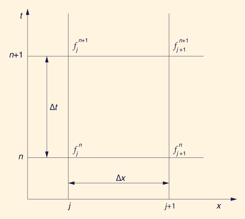
The four-point implicit scheme is based on the following formulas (5), Fig. 1:
in which ƒ(x,t) is any dependent variable; Δx and Δt are the space and time increments; and θ is the weighting factor of the implicit scheme. The weighting factor θ is introduced in the function and its space derivative to allow greater flexibility in the actual operation of the model. While the stable range is 0.5 ≤ θ ≤ 1.0, a strongly stable range is 0.6 ≤ θ ≤ 1.0. The substitution of Eqs. 7-9 into 3 and 4 leads to discretized equations in u' and d'. The solution is postulated in the following exponential form:
in which x* = xSo / do; t* = tuoSo / do and β*R = 2πdo / TuoSo, and u* and d* are dimensionless amplitude functions. The substitution of Eqs. 10 and 11 into the discretized equations in u' and d' yields:
in which i = √-1; ξ = [exp (-iβ* Δt*) - 1 ]; α = σ*Δx* / 2; Δt* = Δt uo So / do and Δx* = Δx So / do. Equations 12 and 13 constitute a set of two homogeneous equations in u* and d*. For the solution to be nontrivial, the determinant of the coefficient matrix must vanish. Accordingly:
in which C / c* = Δt* / Δx*. The value C is referred to as the Courant number, and it is defined as the ratio of the physical celerity c to the "grid celerity" Δx / Δt. Equation 14 is a complex quadratic in ξ.
in which:
and
Calling:
and solving the quadratic Eq. 15, the two roots are:
in which:
and
Since ξ = [exp ( -i β* Δt* ) - 1], it follows that:
and
The dimensioness celerity of the numerical solution c*n is defined as follows (8):
or likewise:
The logarithmic decrement of the numerical solution δn is defined as follows (8):
Since c* is a function of Fo and σ*, and M and N are functions of Fo, σ*, α, C, and θ, it follows that c*n and δn are also functions of Fo, σ*, α, C and θ. Fo and σ* are the physical parameters, Fo being the Froude number and σ* a dimensionless wave number (σ* = 2πdo / LSo). The values α, C, and θ are the numerical parameters, in which α is the spatial resolution (α = π Δx / L); C is the Courant number (C = c Δt / Δx); and θ is the weighting factor of the implicit scheme.
5. CONVERGENCE ANALYSIS
The convergence analysis is based on the following ratios:
The value R1 is the attenuation ratio and R2 is the translation ratio. For R1 > 1, the numerical damping is smaller than the physical damping; for R1 < 1, the numerical damping is greater than the physical damping. For R2 > 1, the numerical translation is greater than the physical translation; and for R2 < 1, the numerical translation is smaller than the physical translation. For R1 = R2 = 1, there is an exact coincidence between analytical and numerical solutions.
The sensitivity of the convergence ratios to the physical and numerical parameters has been studied by varying the parameters within a specified range. For the Froude number Fo, the following range has been studied: 0.01 ≤ Fo ≤ 0.99. This excludes the critical and supercritical regimes. For the wave number σ*, the following range has been studied: 0.01 < σ* < 1,000. This range includes both the kinematic and diffusion waves (σ* ≅ 0.01), and the inertia-pressure waves (σ* ≅ 1,000). The spatial resolution has been varied between π / 100 ≤ α ≤ π / 10. This range includes both a very poor resolution (α ≅ π / 10) and a very high resolution (α ≅ π / 100). The Courant number has been varied in the range 0.25 ≤ C ≤ 4.0. The weighting factor θ has been varied in the range 0 ≤ θ ≤ 1.
The analysis has been performed for the primary wave only (8), by taking the minus sign associated with D and E in Eqs. 30 and 31. Space limitations preclude a complete analysis of both primary and secondary components of the wave propagation.
Figures 2(a)-2(c) portray the attenuation ratio R1 as a function of Fo, σ*, α, C, and θ.
The following general conclusions are obtained from Fig. 2:
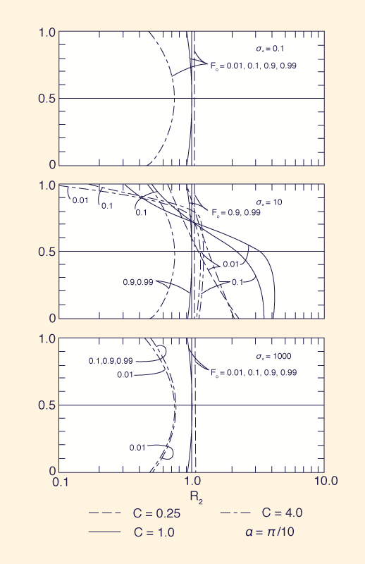
The analysis of the translation ratio R2 shows that this ratio is nearly unity for a wide range of parameters Fo, σ*, α, and C. Predictably, for midrange dimensionless wavenumbers (σ* = 10) and poor spatial resolution, the ratios R2 depart from unity. As an illustration of this trend, Fig. 3 shows the values of R2 for varying Fo, σ*, C, and θ, and α = π / 10.
6. SUMMARY AND CONCLUSIONS
A comprehensive theoretical treatment of the convergence of the four-point implicit numerical model of shallow water waves is presented. The propagation celerity and attenuation factor of the numerical analog are derived, and convergence is tested by establishing the ratio of attenuation and translation given by the numerical and analytical solutions. Convergence is shown to be a function of the complex interaction of five parameters: (1) The Froude number of the equilibrium flow Fo;
The convergence analysis is carried out for Froude numbers in the subcritical regime. Furthermore, due to space limitations, only the primary wave convergence is analyzed.
The following conclusions are warranted by this study:
The simulation is reasonably good for small σ* (kinematic / diffusion) waves and for large σ* (inertia-pressure) waves, provided sufficient care is exercised to minimize the amount of numerical damping.
For intermediate waves σ* (dynamic waves, in which both friction and inertia predominate), the accuracy of the simulation is highly dependent on the correct value of the weighting factor θ.
Values of θ < 0.5 always cause numerical amplification; values of 0.5 ≤ θ < 1 may cause numerical amplification or attenuation; a value of θ = 1 always causes numerical attenuation.
7. LIMITATIONS AND APPLICATIONS
The findings of this study have been obtained by using a linearized version of the Saint Venant equations. Therefore, emphasis should be placed on the qualitative nature of the results. At present, the performance of a nonlinear model can only be assessed through carefully designed numerical experiments. The linear analysis presented herein provides an appropriate framework for the design of these experiments.
8. ACKNOWLEDGMENTS
The research subject of this paper was supported in part by the Colorado State University Experiment Station. Horst Indlekofer was awarded a NATO fellowship to make possible his visit to Colorado State University.
APPENDIX Ι - EQUATIONS FOR PROPAGATION CELERITY c* AND LOGARITHMIC DECREMENT δ OF SINUSOIDAL PERTURBATIONS IN OPEN CHANNEL FLOW (8)
The equations are: c* = 1 ± D; δ = -2π (B ∓ E)/(|1 ± D |), in which A = (1/Fo2) - B2; B = 1/(σ* Fo2);
APPENDIX ΙΙ. REFERENCES
Chaudhry, Y. M., and D. N. Contractor. 1973. "Application of the Implicit Method to Surges in Open Channels," Water Resources Research, Vol. 9, No. 6, Dec., 1605-1612.
Cunge, J. A., and M. Wegner. 1964. "Numerical Integration of the Saint Venant Equations by an Implicit Finite Difference Scheme," La Houille Blanche, Grenoble, France, Vol. 19, No. 1, Jan., 33-39.
Fread, D. L. 1974. "Numerical Properties of Implicit Four-Point Finite Dfference Equations of Unsteady Flow," NOAA Technical Memorandum NWS HYDRO-18, National Oceanic and Atmospheric Administration, Mar.
Liggett, J. A. 1975. "Basic Equations of Unsteady Flow," Unsteady Flow in Open Channels, K. Mahmood and V. Yevjevich, eds., VoL. I, Water Resources Publications, Fort Collins, Colo.
Liggett, J. A., and J. A. Cunge. 1975. "Numerical Methods of Solution of the Unsteady Flow Equations," Unsteady Flow in Open Channels, K. Mahmood and V. Yevjevich, eds., Vol. I, Water Resources Publications, Fort Collins, Colo.
Lighthill, M. J., and G. B. Whitham. 1955. "On Kinematic Waves I, Flood Movements in Long Rivers," Proceedings, Royal Society of London, Vol. A 229, May, 281-316.
O'Brien, G. G., M. A. Hyman, and S. Kaplan. 1950. "A Study of the Numerical Solution of Partial Differential Equations," Journal of Mathematics and Physics, Vol. 29, No. 4, 223-251.
Ponce, V. M., and D. B. Simons. 1977. "Shallow Wave Propagation in Open Channel Flow," Journal of the Hydraulics Division, ASCE, Vol. 103, No. HY12, Proc. Paper 13392, Dec., 1461-1476.
Price, R. K. 1974. "Comparison of Four Numerical Methods of Flood Routing," Journal of the Hydraulics Division, ASCE. Vol. 100, No. HY7, Proc. Paper 10659, July, 879-899.
Quinn, F. H., and E. B. Wylie. 1972. "Transient Analysis of the Detroit River by the Implicit Method," Water Resources Research, Vol. 8, No. 6, Dec., 1461-1469.
Roache, P. J. 1972. Computational Fluid Dynamics, Hermosa Publishers, Albuquerque, NM.
APPENDIX ΙΙΙ. NOTATION
The following symbols are used in this paper:
A, B, C, D, E = parameters, Eqs. 24-28;
a = wave amplitude;
C = Courant number;
c = wave celerity;
d = flow depth;
Fo = Froude number;
ƒ = function;
g = acceleration of gravity;
i = √-1;
j = space discretization index;
L = wavelength;
M, Mo, M1, M2 = parameters;
N, No, N1, N2 = parameters;
n = time discretization index;
P, Q = parameters;
R1 = attenuation convergence ratio;
R2 = translation convergence ratio;
Sƒ = friction slope;
So = bed slope;
T = wave period;
t = time variable;
to = initial time;
u = mean velocity;
x = space variable;
α = spatial resolution parameter;
β* = complex propagation factor;
β*i = imaginary part of β*;
β*R = real part of β*;
Δx = space step;
Δt = time step;
δ = logarithmic decrement;
θ = weighting factor; and
σ* = dimensioinless wavenumber.
Subscripts
o = equilibrium flow; and
n = numerical.
Superscripts
' = perturbed component; and
* = dimensionless parameter / variable.
|

| 220701 18:30 |
| Documents in Portable Document Format (PDF) require Adobe Acrobat Reader 5.0 or higher to view; download Adobe Acrobat Reader. |