1. INTRODUCTION
There are two formulations for hydraulic diffusivity in diffusion wave modeling: the kinematic hydraulic diffusivity (Hayami, 1951) and the dynamic hydraulic diffusivity (Dooge, 1973; Dooge et al, 1982; Ponce, 1991a, 1991b). The kinematic hydraulic diffusivity is: νk = qo/(2So), in which
2. BACKGROUND
Wooding (1965) pioneered the use of kinematic waves in an "open-book" configuration to simulate overland flow. Since then, kinematic waves have become well established in hydrologic research and practice (HEC-1, Flood Hydrograph Package, 1990). However, kinematic waves are nondiffusive; therefore, they should not be used to model situations in which diffusion plays a significant role. The amount of diffusion is controlled by the bottom slope; the steeper the slope the lesser the diffusion, and vice versa. In an urban setting, where plane and channel slopes are typically greater than one percent, diffusion vanishes and kinematic waves prevail. Unfortunately, numerical solutions of kinematic waves introduce varying amounts of "numerical diffusion," masking the true nondiffusive behavior of kinematic waves (Ponce, 1991a).
To cope with this difficulty, Ponce (1986) has proposed a diffusion wave model of overland flow based on the Muskingum-Cunge method. Unlike conventional overland flow kinematic wave models, the Muskingum-Cunge diffusion wave model has the advantage that it incorporates the physical diffusion, if any, of the surface runoff, matching it with the numerical diffusion of the problem at hand. A significant feature of this type of modeling is that it provides grid independence, i.e., the results are not a function of grid size. This frees the model user to concentrate on the physical, rather than on the numerical aspects of the problem, leading to more consistent and better modeling.
The Muskingum-Cunge model is based on the matching of physical and numerical diffusivities. The physical diffusivity is (Hayami, 1951):
The numerical diffusivity is (Cunge, 1969):
in which c = wave celerity, Δx = space interval, and X = Muskingum weighting factor (Chow, 1959). Equating physical and numerical diffusivities leads to
and to
in which
is the cell Reynolds number (Ponce and Yevjevich, 1978).
In Muskingum routing,
in which K = travel time. In Muskingum-Cunge routing,
in which C = Courant number (Ponce and Yevjevich, 1978), and Δt = time interval. Hayami's expression for the hydraulic diffusivity is in essence a kinematic hydraulic diffusivity νk, since inertia is explicitly absent from its formulation.
By including inertia in the formulation of diffusion waves, Dooge (1973) was able to express the hydraulic diffusivity in terms of the Froude number:
in which v = mean velocity, g = gravitational acceleration, and d = hydraulic depth. Dooge's hydraulic diffusivity is:
applicable to the case of Chezy friction in hydraulically wide channels.
Dooge et. al. (1982) generalized this formulation for any friction type and cross-sectional shape:
in which β = exponent of the reataing Q = αAβ, with Q = discharge, and A = flow area.
Dooge's model is a diffusion wave model with inertia, to be distinguished from a dynamic wave model, which entails the complete solution of the governing equations of continuity and motion (the Saint Venant equations). Dooge's (and Dooge et al's) expression for hydraulic diffusivity can properly be regarded as a dynamic hydraulic diffusivity νd, since it does include inertia in its formulation.
Ponce (1991a, 1991b) enhanced Dooge et al's formulation by expressing the dynamic hydraulic diffusivity in terms of the Vedernikov number:
The Vedernikov number [V=(β - 1)F] is the ratio of the relative kinematic wave celerity
Ponce's modification to Hayami's and Dooge's expressions is substantive because it renders the hydraulic diffusivity responsive to the flow dynamics. In effect, for Vedernikov number V = 1, the hydraulic diffusivity vanishes and the flow is on the threshold of neutral stability.
For overland flow applications, the question remains whether the dynamic hydraulic diffusivity does indeed constitute a significant improvement over the kinematic hydraulic diffusivity. Although more appealing from a theoretical standpoint, it has been argued that the dynamic hydraulic diffusivity represents only a small improvement over its kinematic counterpart when practical applications are considered (Perumal, 1992). Therefore, there is a need to clarify the precise role of the Vedernikov number in overland flow dynamics.
3. EXPERIMENTAL PROGRAM
The work reported here set out to compare results of the Muskingum-Cunge diffusion wave overland flow model using: (1) the kinematic cell Reynolds number D, Eq. 5; and (2) the dynamic cell Reynolds number Dd, Eq. 12. In essence, it sought to determine the effect of the Vedernikov number in overland flow dynamics under a wide range of flow conditions (geometry and bottom friction, plane/channel slopes, and effective rainfall intensity). The comparison was undertaken using OVERLAND, a Muskingum-Cunge diffusion wave overland flow model developed by the senior author (Ponce, 1989b). A special version of the model was implemented to handle either the kinematic or dynamic versions of the cell Reynolds number.
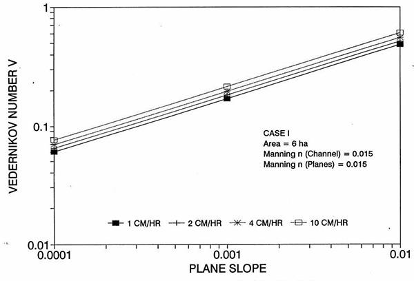
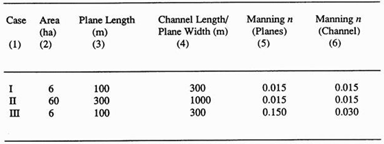
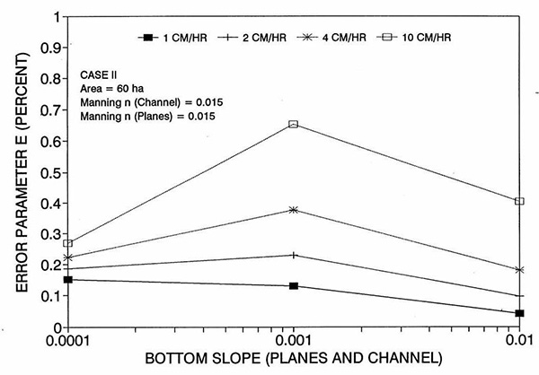
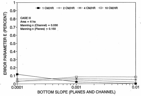
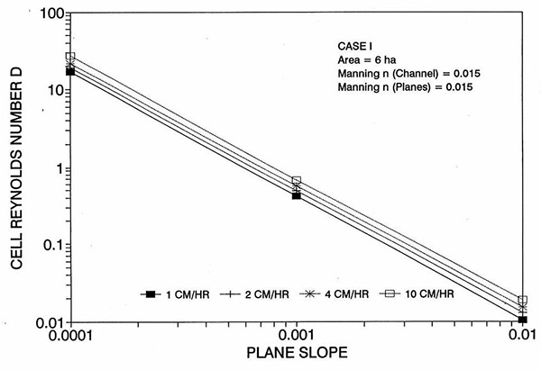
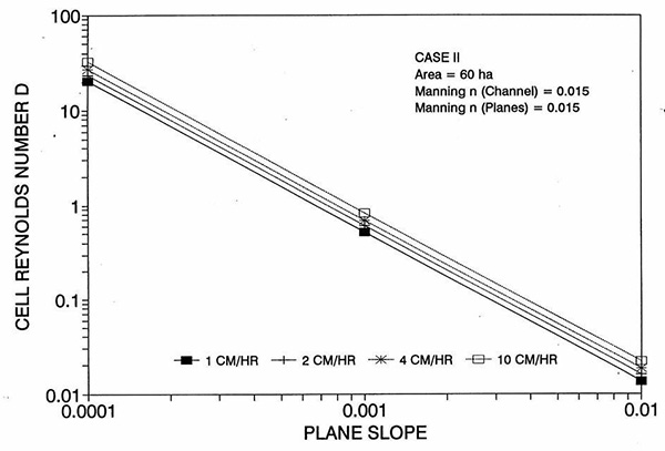
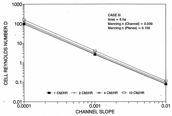
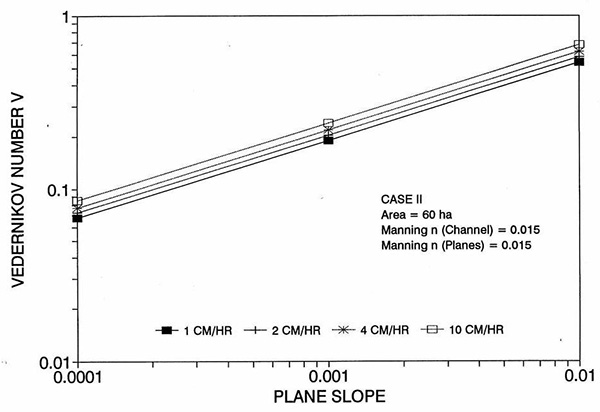
The program of numerical experiments encompassed the three cases shown in Table 1. Case I is a small catchment (6 ha) with low friction (Manning n = 0.015); Case II is a larger catchment (60 ha) with low friction (Manning n = 0.015); Case III is a small catchment (6 ha) with high friction (Manning n = 0.150 in the planes; n = 0.030 in the channel). For each case, three plane/channel slopes were specified: So = 0.01 (steep), So = 0.001 (intermediate), and So = 0.0001 (mild). For each case and for each plane/channel slope, four effective rainfall intensities were specified: ie = 1, 2, 4, and
The input to OVERLAND is effective rainfall intensity ie (cm/hr) lasting a specified duration tr (hr). The output is an outflow hydrograph showing discharge (m3/sec) vs time (hr). For each run, the rainfall duration was carefully chosen to allow the outflow to reach equilibrium, at which time the rainfall ceased and the flow gradually receded to zero. The discharge at equilibrium is: Qe = ieA, in which A = catchment area (Ponce, 1989a). 4. RESULTS The results of the simulations showed a small but perceptible lag in the rising limb of the outflow hydrograph, coupled with a corresponding lag in the receding limb, when comparing runs using kinematic and dynamic cell Reynolds numbers. The existence of the lag is attributed to the error of the kinematic solution, which used the original formulation of the cell Reynolds number (Eq. 5), as opposed to the dynamic solution, which relied on the enhanced Vedernikov-number-dependent formulation (Eq. 12). The error was quantified by integrating the absolute value of the difference between the two hydrographs, kinematic and dynamic, to obtain a runoff volume difference ΔV:
The runoff volume difference was normalized by dividing it by the total runoff volume Vr = ie tr A. Therefore, the error E (in percent) is:
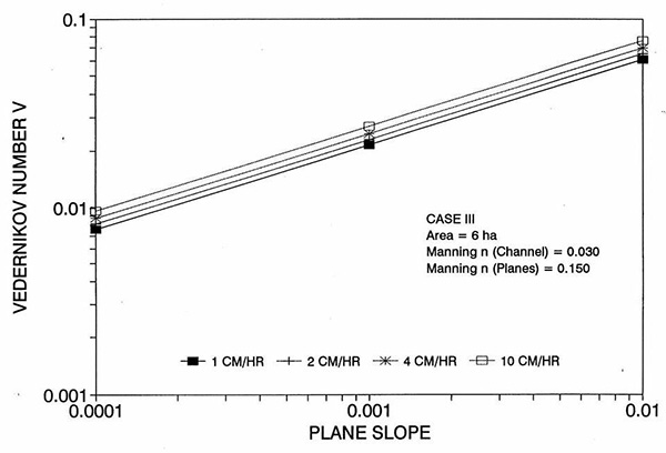
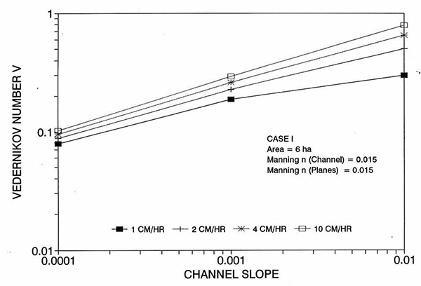
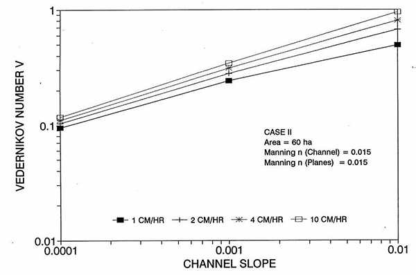
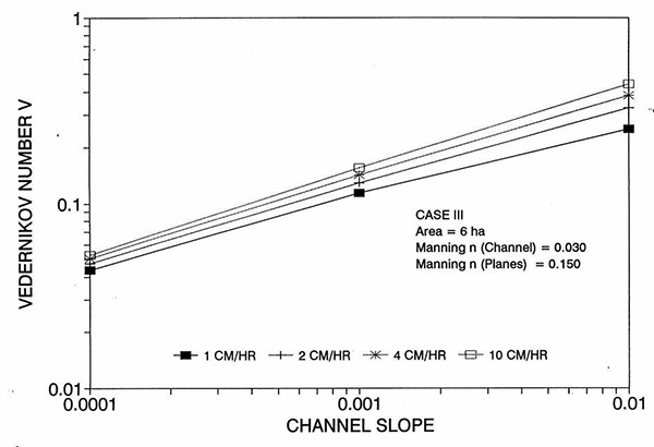
Figure 1 shows the error incurred by using a kinematic cell Reynolds number in a diffusion wave overland flow solution, as a function of bottom slope, for each of three cases: (a) Case Ι, (b) Case ΙΙ, and (c) Case ΙΙΙ. These results show that the error is indeed small but perceptible, and likely to remain within 0.7 percent for a wide range of flow conditions. This figure also shows that the error is inversely related to bottom friction: for Cases I and II, the error is less than 0.7 percent for rainfall intensities less than 10 cm/hr; for Case ΙΙΙ it is typically less than 0.1 percent. The results also show a tendency for the error to peak around the midrange of bottom slopes (So = 0.001). 5. ANALYSIS The tendency for the error to peak around the midrange of bottom slopes requires further discussion. Figures 2 and 3 show the variation of the cell Reynolds number D with plane and channel slope, respectively. Figures 4 and 5 show the variation of the Vedernikov number V with plane and channel slope, respectively. The following conclusions can be drawn from these figures:
These findings underscore the futility of attempting to model overland flow by resorting to the complete hydrodynamic equations (Chow and Ben-Zvi, 1973; Tayfur et al, 1993). Since the diffusion wave model with inertia does not substantially improve the description of the wave dynamics for a wide range of flow conditions, it follows that there is very little to be gained by pursuing an even more precise and elaborate formulation. Moreover, since the diffusion wave model with inertia does not unduly complicate the formulation, it should be the preferred way of modeling overland flow with diffusion waves. 6. SUMMARY A program of numerical experiments has been performed to test the effect of the dynamic hydraulic diffusivity (Dooge, 1973; Ponce, 1991b) vis-à-vis the kinematic hydraulic diffusivity (Hayami, 1951), when used to model overland flow with diffusion waves. Two models (a conventional diffusion wave and a diffusion wave with inertia), three typical open-book overland flow scenarios of distinct geometry and bottom roughness, three bottom slopes (steep, intermediate, and mild), and four effective rainfall intensities (1, 2, 4, and 10 cm/hr) led to a total of 72 computer runs using a Muskingum-Cunge overland flow model. Results showed a small but perceptible lag in the rising limb of the outflow hydrograph, coupled with a corresponding lag in the receding limb, when comparing inns using the two competing models. The lag is attributed to the error of the kinematic solution, which is based on the kinematic cell Reynolds number [ D = qo/(So c Δx) ], as compared to the dynamic solution, which bases the calculation of diffusion on the dynamic cell Reynolds number [ Dd = (1 - V2)D ]. The error was evaluated by integrating the absolute value of the difference between the two hydrographs, to obtain a runoff volume difference, which was normalized by dividing it by the total runoff volume. The results show that the error is indeed small but perceptible, and likely to remain within 0.7 percent for a wide range of flow conditions. The results also show a tendency for the error to peak around the midrange of bottom slopes (So = 0.001). The findings of this study underscore the futility of attempting to model overland flow by using the complete hydrodynamic equations. Since the dynamic effect is shown to be small throughout a wide range of bottom slopes, a diffusion wave model with inertia may be all that is required to model the overland flow dynamics. Moreover, since the diffusion wave model with inertia does not unduly complicate the formulation, it should be the preferred way of modeling overland flow using diffusion waves. REFERENCES
Chow, V. T., and A. Ben-Zvi. 1973. "Hydrodynamic Modeling of Two-dimensional Watershed Flow." Journal of the Hydraulics Division, ASCE, 99(11), 2023-2040.
Craya, A. 1952. "The Criterion of the Possibility of Roll Wave Formation." Gravity Waves, National Bureau of Standards Circular No. 521, 141-151.
Cunge, J. A. 1969. "On the Subject of a Flood Propagation Computation Method (Muskingum Method)." Journal of Hydraulic Research, 7(2), 205-230.
Dooge, J. C. I. 1973. Linear Theory of Hydrologic Systems. Tech. Bull., No. 1468, USDA Agricultural Research Service, Washington, D.C..
Dooge, J. C. I., W.., Strupczewski, and J. J. Napiorkowski. 1982.
"Hydrodynamic Derivation of Storage Parameters in the Muskingum Model." Journal of Hydrology, 54, 371-387.
Hayami, S. 1951. "On the Propagation of Flood Waves." Bulletin Disaster Prevention Research Institute, Kyoto University, 1(1), 1-16.
HEC-1, Flood Hydrograph Package: User's Manual. 1990. U.S. Army Corps of Engineers, Hydrologic Engineering Center, Davis, Calif., September.
Perumal, M. 1992. Comment on "New Perspective on the Vedernikov Number." Water Resources Research, 28(6), 1735.
Ponce, V. M., and D. B. Simons.. 1977. "Shallow Wave Propagation in Open Channel Flow." Journal of the Hydrauclis Division, ASCE, 103(12), 1461-1476.
Ponce, V. M., and V. Yevjevich, V. 1978. "Muskingum-Cunge Method with Variable Parameters." Journal of the Hydraulics Division, ASCE, 104(12), 1663-1667.
Ponce, V. M. 1986. "Diffusion Wave Modeling of Catchment Dynamics." Journal of Hydraulic Engineering, ASCE, 112(8), 716-727.
Ponce, V. M. 1989a. Engineering Hydrology, Principles and Practices. Prentice Hall, Englewood Cliffs, New Jersey.
Ponce, V. M. 1989b. "Diffusion Wave Overland Flow Module." Technical Report prepared for USGS Water Resources Division, Stennis Space Center, Miss., June.
Ponce, V. M. 1991a. "The Kinematic Wave Controversy." Journal of Hydraulic Engineering, ASCE, 117(4), 511-525.
Ponce, V. M. 1991b. "New Perspective on the Vedemikov Number." Water Resources Research, 27(7), 1777-1779.
Tayfur, G., M. L. Kavvas, and R. S. Govindaraju. 1993. Applicability of St. Venant Equations for Two-dimensional Overland Flow Over Rough Infiltrating Surfaces. ASCE Journal of Hydraulic Engineering, 119:51-63.
Wooding, R. A. 1965. "A Hydraulic Model for the Catchment-Stream Problem." Journal of Hydrology, 3, 254-267.
NOTATION
A = flow area, catchment area;
C = Courant number;
c = wave celerity;
cri = relative inertial wave celerity (Lagrange celerity);
crk = relative kinematic wave celerity;
D = kinematic cell Reynolds number;
Dd = dynamic cell Reynolds number;
d = hydraulic depth;
do = reference flow depth;
E = percent error;
F = Froude number;
g = gravitational acceleration;
ie = effective rainfall intensity;
K = Muskingum travel time;
L = wavelength;
Lo = reference channel length;
n = Manning roughness coefficient;
Q = discharge;
Qe = equilibrium discharge;
qo = reference unit-width discharge;
So = bottom slope;
t = time variable;
tr = effective rainfall duration;
V = Vedernikkov number;
Vr = total runoff volume;
v = mean velocity;
X = Muskingum weighting factor;
α = coefficient of the rating Q = αAβ;
β = exponent of the rating Q = αAβ;
Δt = time interval;
Δx = space interval;
ΔV = runoff volume difference;
ν = hydraulic diffusivity;
νd = dynamic hydraulic diffusivity;
νk = kinematic hydraulic diffusivity; and
σ = dimensionless wave number.
|


| 221230 |
| Documents in Portable Document Format (PDF) require Adobe Acrobat Reader 5.0 or higher to view; download Adobe Acrobat Reader. |