QUESTIONS
- Describe the frontal lifting of air masses.
|
Frontal lifting takes place when relatively warm air flowing toward a colder air mass is forced upward, with the cold air acting as a wedge. Cold air overtaking warmer air will produce the same result by "wedging" the latter aloft. The surface of separation between the two different air masses is called a frontal surface.
|
- What is orographic lifting? What is thermal lifting?
|
Orographic lifting occurs when air flowing towards an orographic barrier (i.e., mountain) is forced to rise in order to pass over it.
Thermal lifting is caused by local heating. As heated surface air becomes buoyant, it is forced to rise, resulting in its cooling. If the local heated air contains enough moisture and rises far enough, saturation will be reached and cumulus clouds will form.
|
- Describe the concept of rainfall frequency.
|
Rainfall frequency refers to the average time elapsed between occurrences of two rainfall events of the same depth and duration.
|
- What is the PMP? What is the PMF?
|
The Probable Maximum Precipitation, or PMP, is the theoretically greatest depth of precipitation for a given geographic location, catchment area, event duration, and time of the year. The Probable Maximum Flood, or PMF, is the flood event associated with the PMP.
|
- In what case is the isohyetal method preferred over the Thiessen polygons method?
|
The isohyetal method is preferred over the Thiessen polygons method when averaging precipitation over catchments where orographic effects have a significant influence on the local storm pattern.
|
- When is an IDF curve used? When is a Depth-Duration-Frequency value used?
|
An intensity-duration-frequency, or IDF, curve is used in small catchment runoff analysis, where the short rainfall duration generally justifies the assumption of constant rainfall intensity.
A depth-duration-frequency rainfall value is used in midsize catchment runoff analysis, together with a chosen temporal storm distribution, to develop the hyetograph for a given storm.
|
- How does average annual precipitation affect climate?
|
Average annual precipitation determines the type of climate that prevails in a given region, either (1) arid, (2) semiarid, (3) sub-humid or (4) humid. An arid climate prevails in regions having less than 400 mm of average annual precipitation. A semiarid climate is found in regions having between 400 and 800 mm of average annual precipitation. A subhumid climate is found in regions having between 800 mm and 1600 mm of average annual precipitation. A humid climate is found in regions with more than 1600 mm of average annual precipitation.
|
- When is the normal ratio method used to fill in missing precipitation records?
|
The normal ratio method is used to fill in missing records from station X when the mean annual rainfall at any of the three index stations A, B, and C differs by more than 10% from that of station X.
|
- What is a double-mass analysis?
|
Double-mass analysis is a procedure to test the consistency of a rainfall record. The method aims at detecting changes in the location or exposure of a rain gage which may have a significant effect on the amount of precipitation it measures.
|
- What type of storm is likely to be subtantially abstracted by interception?
|
Light storms are substantially abstracted by the interception process because a large proportion of the storm goes into interception storage, with very little of it being converted into runoff.
|
- What factors affect the process of infiltration?
|
Infiltration rates depend on:
(1) The condition of the land surface, including compaction and surface crusting,
(2) The type, extent and density of vegetative cover, and associated root structure,
(3) The physical properties of the soil, including grain size and gradation,
(4) The storm character, i.e., intensity, depth, and duration,
(5) The water temperature, and
(6) the water quality, including chemical constituents and other impurities.
|
- Compare the Horton and Philip infiltration formulas.
|
The Horton formula is an exponential decay formula, giving finite values of infiltration rate at time t = 0 and time t = ∞. On the other hand, the Philip formula is a parabolic equation, with infiltration rate at time t = 0 equal to and at time t = ∞ equal to A, a value close to the
saturated hydraulic conductivity. The Horton formula is widely used,
although the decay of infiltration rate with time may not always follow
an exponential function. In spite of the fact that the initial
infiltration rate does have a finite value, the Philip formula seems to
provide a good fit to experimental data.
|
- What type of application justifies the use of a φ-index?
|
The φ-index is best suited for applications involving either
long-duration storms or catchments with high initial soil moisture
content. Under such conditions, the neglect of the variation of
infiltration rate with time is generally justified on practical grounds.
|
- In what case is depression storage likely to be important in runoff evaluation?
|
Depression storage is likely to be important in rainfall-runoff analysis
of low-relief catchments, for instance, low-lying areas, swamps, and the
like. This is because the milder the catchment's relief, the greater the
probability that runoff will be retained in surface depressions.
Consequently, the greater the attenuating effect on the runoff peak.
|
- What is the basis of the energy budget method for determining reservoir evaporation?
|
The energy budget method for determining reservoir evaporation is based
on an accounting of the energy exchanges occurring at the evaporating
surface, including solar radiation and heat transfer from the atmosphere
and from energy stored in the water body.
|
- What is albedo? What is the albedo of a forest? Of a desert?
|
Albedo is the reflectivity coefficient of a surface toward shortwave
radiation, varying with color, roughness, and inclination of the surface.
Typical values of albedo are about 0.03-0.10 for water, 0.05-0.30 for vegetated
areas, 0.15-0.40 for bare soil, and up to 0.95 for snow-covered areas.
The albedo of a forest varies from 0.05 to 0.20. The albedo of a desert varies from 0.20 to 0.45.
|
- What assumptions did Penman use in deriving his evaporation formula?
|
Penman neglected the variations of energy in the water body (Qa = 0 and
Qt = 0) and assumed atmospheric pressure p = 1000 mb. However, the
crucial assumption in Penman's evaporation formula is the calculation of
mass-transfer evaporation rate by assuming that the temperatures of water
surface and overlying air are equal.
|
- What is transpiration? Why is it considered a hydrologic abstraction?
|
Transpiration is the process by which plants transfer water from the root
zone to the leaf surface, where it eventually evaporates into the
atmosphere. Transpiration is considered to be a hydrologic abstraction
because it is an intrinsic part of evapotranspiration, by which moisture
is transferred from the root zone to the atmosphere. Evaporation fran
vegetative surfaces cannot occur continuously without the aid of
transpiration.
|
- What is potential evapotranspiration? What is actual evapotranspiration?
|
Potential evapotranspiration is the amount of evapotranspiration that would take place under the assumption of an ample supply of moisture at all times.
Actual evapotranspiration is the amount of evaporatransration that would take place when water is limiting.
|
- What is reference crop evapotranspiration?
|
Reference crop evapotranspiration is the rate of evaporation from an extended surface of 8 to 15-cm tall green grass cover of uniform height, actively growing, completely shading the ground, and not short of water.
|
- What is the rationale for using evaporation formulas in the evaluation of evapotranspiration?
|
Evaporation and evapotranspiration generally obey the same physical
principles and correlate with the same meteorological variables. For
instance, the Penman formula is commonly used to calculate either
evaporation or evapotranspiration. The radiation and mass-transfer
components of the Penman formula tend to compensate each other. The
radiation component is greater for free water surface evaporation,
whereas the mass-transfer component appears to be greater for potential
evapotranspiration.
|
- What are the various types of surface flow that can occur in nature?
|
Surface flow in catchment can occur as a progression of the following
forms: (1) overland flow, (2) rill flow, (3) gully flaw, (4) streamflow,
and (5) river flow.
|
- What is a hypsometric curve? When is it used?
|
A hypsometric curve is a dimensionless curve showing the variation with
elevation of the catchment subarea above that elevation. It is used to
describe the effect of altitude on hydrologic or climatic variables, for
instance, vegetation cover, snow cover, and the like.
|
- Derive the formula for equivalent slope (Eq. 2-52). State any assumptions used.
|
According to the Manning or Chezy equations, mean velocity is proportional to the square root of channel slope. As an approximation, assume constant hydraulic radius and Manning friction. Then the time of travel in each subreach is:
Li
ti = __________
k Si1/2
|
in which k = (1/n) R 2/3.
The total time of travel through all subreaches is:
n
Σ Li
i = 1
tt = ___________________
n
k Σ Si 1/2
i = 1
|
According to the Manning or Chezy equations, the total time of travel in terms of the equivalent slope S3 is:
n
Σ Li
i = 1
tt = ___________________
k S3 1/2
|
The equation for equivalent slope (Eq. 2-52) is obtained by solving for S3 from the two equations for total time of travel.
n
Σ Li
i = 1
S3 = [ _______________ ] 2
n
Σ ( Li /
Si 1/2 )
i = 1
|
|
- What is interflow? What is groundwater flow?
|
Interflow is subsurface flow, i.e., flow that takes place in the unsaturated soil layers located beneath the ground surface. Groundwater flow takes place below the groundwater table in the form of saturated flow through alluvial deposits and other water-bearing formations located beneath the soil mantle. Groundwater flow includes the portion of infiltrated volume that has reached the water table by percolation from the overlying soils.
|
- What is direct runoff? What is indirect runoff?
|
Direct runoff, or surface flow, is runoff produced by effective rainfall. Indirect runoff is surface runoff originating in interflow and groundwater flow. Baseflow is a measure of indirect runoff.
|
- How does an ephemeral stream differ from an intermittent stream?
|
An ephemeral stream has flow only in direct response to effective precipitation, i.e., during and immediately following a major storm.
Perennial streams always have flow. The dry-weather flow of perennial streams is baseflow originating in groundwater. An intermittent stream is one behaving as perennial at certain times of the year and as ephemeral at other times.
|
- Why is the catchment's antecedent moisture important in flood hydrology?
|
The catchment's antecedent moisture is important in flood hydrology
because it determines to a large extent the type of catchment response.
Wet antecedent moisture causes very little abstraction, resulting in
large amounts of surface runoff and, consequently, large peak flows. Dry
antecedent moisture results in substantial amounts of abstraction and,
consequently, small quantities of surface runoff.
|
- What is catchment response? What is runoff concentration? What is runoff diffusion?
|
Catchment response is the rate and volume of runoff produced at the catchment outlet and caused by a given precipitation excess, or effective rainfall.
Runoff concentration is the property of catchment runoff by which the
flow rate at the catchment outlet increases gradually in response to
effective precipitation, until the entire catchment has had a chance to
contribute to the flow at the outlet. At that time the maximum, or
equilibrium, flow rate is reached at the catchment outlet.
Runoff diffusion is the property of catchment runoff which has the net
effect of smoothing out catchment response, making it a continuous
function. In practice, runoff diffusion acts to spread the hydrograph in
time, reducing flow rates to levels below those which could be attained
by runoff concentration only.
|
- Why do single-storm streamflow hydrographs generally exhibit a long tail?
|
The long tail generally exhibited by single-storm streamflow hydrographs
is due to the markedly different response characteristics of surface
runoff, interflow, and groundwater flow. Surface runoff is fast and
peaked; interflow and groundwater flow are slow and subdued. The
superposition in time of these three runoff components results in a
hydrograph showing a long tail.
|
- Why is the Manning equation preferred over the Chezy equation in practice?
|
The Manning equation is preferred over the Chezy equation because in natural channels the Chezy coefficient is not constant, tending to increase with hydraulic radius:
This equation implies that the Manning n value is a constant. Experience
has shown, however, that the value of n may vary with discharge,
especially in the case of alluvial rivers.
|
- What is the advantage of the Chezy equation?
|
Unlike the Manning equation, the Chezy equation has the advantage that it
can be readily expressed in dimensionless form.
|
- Discuss low flows and high flows in connection with arid and humid climates.
|
In arid climates, low flows are small because the contribution from
groundwater to baseflow is small or almost nonexistent. In humid
climates, low flows are substantial because the contribution from
groundwater to baseflow is large and continuous in time. In arid
climates, because of the small baseflow, the ratio of high flow to low
flow is likely to be very large. In humid climates, because of the
relatively high baseflow and groundwater replenishment, the ratio of high
flow to low flow is not likely to be very large.
|
- What is a rating curve? What are the various processes likely to affect a rating?
|
A rating curve is a relationship between stage and discharge at a certain
location in a stream or river. The processes likely to affect the rating
are: (1) flow nonuniformity (i.e., gradually varied steady flow), (2)
flow unsteadiness (i.e., gradually varied unsteady flow), (3) the
short-term variation of boundary friction with flow rate, and (4) the
long-term cycles of erosion and deposition in stream and river beds.
|
- How can seasonal and annual streamflow variability be explained?
|
The reason for the seasonal and annual variability of streamflow lies in
the relative contributions of direct and indirect runoff. Groundwater
reservoirs serve as the mechanism for the storage of large amounts of
moisture, which are slowly transported to lower elevations. Some of this
moisture is eventually released back to the surface waters. The net
effect is that of a permanent contribution from groundwater to surface
water in the form of dry-weather flow. To evaluate the seasonal and
annual variability of streamflow, it is necessary to examine the relation
between surface water and groundwater.
|
- What is the reason for the high peaks and low valleys of typical daily streamflows of small upland catchments?
|
Small upland catchments are likely to have steep gradients and,
therefore, to concentrate flows with negligible runoff diffusion,
producing hydrographs which show a large number of high peaks with
correspondingly low valleys.
|
- What is a flow-duration curve? For what is it used?
|
A flow-duration curve is a plot showing the permanence of characteristic
low-flow levels. It is useful in the planning and design of water
resources projects, particularly for those projects where it is necessary
to ascertain the permanence of characteristic low-flow levels, for
instance, hydropower generation from a run-of-the-river plant.
|
- What is a flow-mass curve? For what is it used?
|
A flow-mass curve is a plot showing cumulative values of runoff volumes
(in the ordinates) versus time (in the abscissas). It is used in the
study of streamflow variability, whether seasonal or annual, particularly
in the determination of the adequate size of storage reservoirs.
|
- What is the Hurst phenomenon?
|
The Hurst phenomenon is the name given to the discrepancy between theory
and experimental data with regard to the exponent for the equation
defining range. Whereas measurements show a mean value of the exponent
of 0.73, theory indicates that the value should be 0.5.
|
- How does peak discharge per unit area vary with catchment size? Why?
|
Peak discharge per unit area varies inversely with catchment size. The
reason for this is that in general, the greater the catchment, the
smaller the overall catchment slope, and consequently, the greater the
likelihood that hydrologic abstractions and runoff diffusion will act to
decrease and/or attenuate peak discharge.
|
PROBLEMS
A 465-km2 catchment has mean annual precipitation of 775 mm and mean annual flow of 3.8 m3/s.
What percentage of total precipitation is abstracted by the catchment?
|
The mean annual flow is:
|
3.8 m3/s × 86,400 s/d × 365 d/y × 1000 mm/m
Q = ___________________________________________________
= 257.7 mm/y
465 km2 × (1000 m/km)2
The percentage of total precipitation abstracted by the catchment is:
[(775 - 257.7)/ 775] × 100 = 66.7 percent. ANSWER.
|
|
A 9250-km2 catchment
has mean annual precipitation of 645 mm and mean annual flow of 37.3 m3/s. What is the precipitation
depth abstracted by the catchment?
|
The mean annual flow is:
|
37.3 m3/s × 86,400 s/d × 365 d/y × 1000 mm/m
Q = ___________________________________________________
= 127.2 mm/y
9250 km2 × (1000 m/km)2
The precipitation depth abstracted by the catchment is equal to:
(645 - 127.2) = 517.8 mm/y. ANSWER.
|
|
Using the dimensionless temporal rainfall distribution
shown in Fig. 2-5, calculate a hyetograph for an 18-cm, 12-h storm, defined at l-h intervals.
|
The hyetograph defined at 1-h intervals is shown below:
Time
(h) |
Percentage depth
(from Fig. 2-5) |
Incremental
percentage |
Rainfall depth
per increment
(cm) |
| 0 |
0 |
- |
0.0 |
| 1 |
5 |
5 |
0.9 |
| 2 |
10 |
5 |
0.9 |
| 3 |
15 |
5 |
0.9 |
| 4 |
20 |
5 |
0.9 |
| 5 |
30 |
10 |
1.8 |
| 6 |
40 |
10 |
1.8 |
| 7 |
55 |
15 |
2.7 |
| 8 |
70 |
15 |
2.7 |
| 9 |
80 |
10 |
1.8 |
| 10 |
90 |
10 |
1.8 |
| 11 |
95 |
5 |
0.9 |
| 12 |
100 |
5 |
0.9 |
| Sum |
|
100 |
18.0 |
|
|
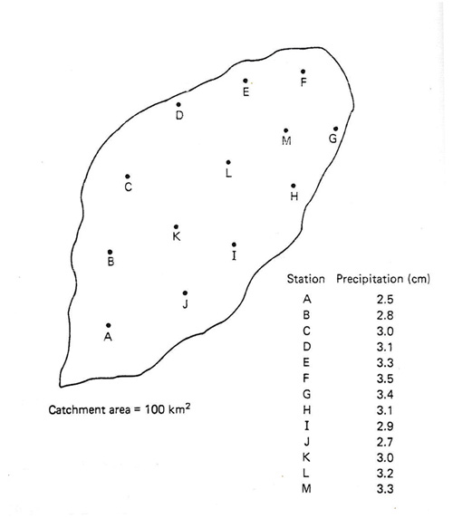
A 100-km2
catchment is instrumented with 13 rain gages located as shown in Fig. M-2-4b.
Immediately after a certain precipitation event, the rainfall amounts accumulat
ed in each gage
are as shown in the figure. Calculate the average precipitation over the catchment by the following methods:
(a) average rainfall, (b) Thiessen polygons, and (c) isohyetal method.
|
Fig. M-2-4 Spatial distribution of rain gages for Problem 2-4.
|
|
(a) Average rainfall: The sum of all station precipitation values
divided by the number of stations:
Pa= Σ P/13 = 39.8/13 = 3.06 cm.
ANSWER.
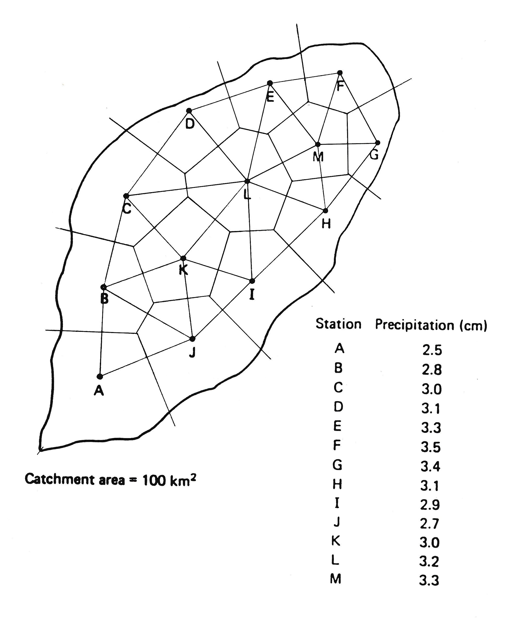
(b) Thiessen Polygons: As shown in Fig. M-2-4(b) and detailed below.
|
Fig. M-2-4b Solution by Thiessen polygons.
|
| Station |
Rainfall P
(cm) |
Area A
(km2) |
PA
(cm-km2) |
| A |
2.5 |
13.06 |
32.65 |
| B |
2.8 |
8.86 |
24.81 |
| C |
3.0 |
9.89 |
29.67 |
| D |
3.1 |
6.25 |
19.37 |
| E |
3.3 |
5.04 |
16.63 |
| F |
3.5 |
5.69 |
19.91 |
| G |
3.4 |
4.01 |
13.63 |
| H |
3.1 |
6.53 |
20.24 |
| I |
2.9 |
8.77 |
25.43 |
| J |
2.7 |
9.89 |
26.70 |
| K |
3.0 |
7.46 |
22.38 |
| L |
3.2 |
9.05 |
28.96 |
| M |
3.3 |
5.50 |
18.15 |
| Sum |
|
100 |
298.53 |
|
The average rainfall is: Pa = Σ(PA) / ΣA = 2.985 cm.
ANSWER.
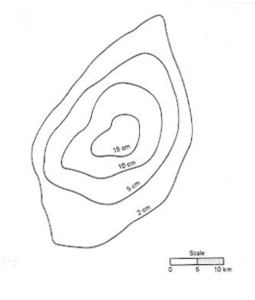
(c) Isohyetal method: As shown in Fig. M-2-4(c) and detailed below.
|
Fig. M-2-4c Solution by isohyetal method.
|
Isohyet P
(cm) |
Area A
(km)2 |
PA
(cm-km2) |
| 2.5 |
11.75 |
29.375 |
| 2.6 |
6.16 |
16.016 |
| 2.7 |
6.72 |
18.144 |
| 2.8 |
8.77 |
24.556 |
| 2.9 |
10.73 |
31.117 |
| 3.0 |
14.56 |
43.680 |
| 3.1 |
13.24 |
41.044 |
| 3.2 |
9.61 |
30.752 |
| 3.3 |
7.83 |
25.839 |
| 3.4 |
5.41 |
18.394 |
| 3.5 |
5.22 |
18.270 |
| Sum |
100 |
297.180 |
|
The average rainfall is: Pa = Σ(PA) / ΣA = 2.97 cm.
ANSWER.
|
A certain
catchment experienced a rainfall event with the following incremental depths:
|
Time (h) | 0-3 | 3-6 | 6-9 | 9-12 |
| Rainfall (cm) | 0.4 | 0.8 | 1.6 | 0.2 |
Determine: (a) the average rainfall
intensity in the first 6 h, (b) the average rainfall intensity for the entire duration of the
storm.
|
(a) The average rainfall intensity in the first 6 hours is:
(0.4 + 0.8) cm /(6 h) = 0.2 cm/h. ANSWER.
(b) The average rainfall intensity for the entire duration of the storm
is:
(0.4 + 0.8 + 1.6 + 0.2) cm /(12 h) = 0.25 cm/h. ANSWER.
|
The following dimensionless temporal rainfall distribution has been determined for
a local storm:
|
Time (%) | 0 | 10 | 20 | 30 | 40 | 50 | 60 | 70 | 80 | 90 | 100 |
| Rainfall depth (%) |
0 | 5 | 10 | 25 | 50 | 75 | 90 | 95 | 97 | 99 | 100 |
Calculate a design hyetograph for a 12-cm, 6-h storm.
Express in terms of hourly rainfall depths.
|
By linear interpolation, the dimensionless temporal rainfall
distribution is converted to match the 6-h storm duration.
|
Time (h) | 0 | 1 | 2 | 3 | 4 | 5 | 6 |
|
Percent time | 0.0 | 16.7 | 33.3 | 50.0 | 66.7 | 83.3 | 100.0 |
|
Percent depth | 0.0 | 8.3 | 33.3 | 75.0 | 93.3 | 97.7 | 100.0 |
The incremental change is obtained by subtracting each percent depth from the previous one:
|
Time (h) | 0 | 1 | 2 | 3 | 4 | 5 | 6 |
|
Incremental percentage | - | 8.3 | 25.0 | 41.7 | 18.3 | 4.4 | 2.3 |
The design hyetograph for the 12-cm 6-h storm is:
|
Time (h) | 0 | 1 | 2 | 3 | 4 | 5 | 6 |
|
Depth (cm) | - | 1 | 3 | 5 | 2.2 | 0.52 | 0.28 |
It is verified that the sum of rainfall depths is equal to 12 cm.
|
Given the following intensity-duration
data, find the a and m constants of Eq. 2-5.
|
Intensity (mm/h) | 50 | 30 |
| Duration (h) | 0.5 | 1.0 |
|
Since i = a / tm, it follows that log i = log a - m log t. Therefore:
log (50)= log a - m log (0.5)
log (30)= log a - m log (1.0)
Solving for a and m: a = 30; m = 0.737. ANSWER.
|
Given the following intensity-duration data, find the constants a and b of Eq. 2-6.
|
Intensity (mm/h) | 60 | 40 |
| Duration (h) | 1 | 2 |
|
Since i = a /(t + b), it follows that:
60 =a /(1 + b); and
40 = a /(2 + b).
Solving for a and b: a = 120; b = 1. ANSWER.
|
Construct a depth-area curve for the 6-h duration
isohyetal map shown in Fig. P-2-9.
|
Fig. P-2-9 Isohyetal map for Problem 2-9.
|
|
The calculations are shown in the following table.
| (1) | (2) | (3) | (4) | (5) | (6) |
Isohyetal
Value
(cm) |
Area
(km2) |
Area
Difference
(km2) |
Volume
(km2-cm) |
Cumulative
Volume
(km2-cm) |
Average
Depth
(cm) |
| 15 |
55.6 |
55.6 |
834. |
834. |
15.00 |
| 10 |
217.8 |
162.2 |
1622. |
2546. |
11.69 |
| 5 |
462.2 |
244.4 |
1222. |
3678. |
7.96 |
| 2 |
831.1 |
368.9 |
738. |
4416. |
5.31 |
|
The areas enclosed within each isohyet (Col. 2) are planimetered from
Fig. P-2-9. The subarea applicable to each isohyetal value is the area
difference (Col. 3). The volume is obtained by multiplying the area
difference (km2 ) by the corresponding isohyetal value (cm). The
cumulative volume (Col. 4) is the sum of all volumes up to the
indicated isohyetal value. For each isohyetal value, the average depth
is the cumulative volume (Col. 5) divided by the area (Col. 2).
Columns 6 and 2 show the depth-area data for the 6-h storm duration.
ANSWER.
|
The precipitation gage for station X was
inoperative during part of the month of January. During that same period, the precipitation
depths measured at three index stations A, B, and C were 25, 28, and 27 mm, respectively.
Estimate the missing precipitation data at X. given the following average annual
precipitation at X, A, B, and C: 285, 250, 225, and 275 mm, respectively.
|
Since the average annual precipitation at station B differs by more
than 10 percent from that of station X, the missing precipitation
record at station X can be estimated by the normal ratio method (Eq.
2-10):
Px = (1/3)[(285/250) × 25 + (285/225) × 28 + (285/275) × 27] =
Px = 30.65 mm. ANSWER.
|
The
precipitation gage for station Y was inoperative during a few days in February. During that
same period, the precipitation at four index stations, each located in one of four
quadrants (Fig. 2-15), is the following:
| Quadrant | Precipitation
(mm) | Distance
(km) |
| I | 25 | 8.5 |
| II | 28 | 6.2 |
| III | 27 | 3.7 |
| IV | 30 | 15.0 |
Estimate the missing precipitation data at station Y.
|
The missing precipitation record at station Y can be estimated with Eq. 2-11. The calculations are shown in the following table.
| Quadrant |
Precipitation P
(mm) |
Distance L
(km) |
1/L2
|
P/L2
|
| I |
25 |
8.5 |
0.01384 |
0.3460 |
| II |
28 |
6.2 |
0.02601 |
0.7283 |
| III |
27 |
3.7 |
0.07304 |
1.9721 |
| IV |
30 |
15.0 |
0.00444 |
0.1332 |
| Sum |
|
|
0.11733 |
3.1796 |
|
Therefore: PY = 3.1796 / 0.11733 = 27.1 mm. ANSWER.
|
The annual precipitation at station Z
and the average annual
precipitation at 10 neighboring stations are as follows:
|
| Year | Precipitation at Z
(mm) | 10-station average
(mm) |
| 1972 | 35 | 28 |
| 1973 | 37 | 29 |
| 1974 | 39 | 31 |
| 1975 | 35 | 27 |
| 1976 | 30 | 25 |
| 1978 | 25 | 21 |
| 1979 | 20 | 17 |
| 1980 | 24 | 21 |
|
| Year | Precipitation at Z
(mm) | 10-station average
(mm) |
| 1981 | 30 | 26 |
| 1982 | 31 | 31 |
| 1983 | 35 | 36 |
| 1984 | 38 | 39 |
| 1985 | 40 | 44 |
| 1984 | 28 | 32 |
| 1985 | 25 | 30 |
| 1985 | 21 | 23 |
|
Use double-mass analysis
to correct for any data inconsistencies at station Z.
|
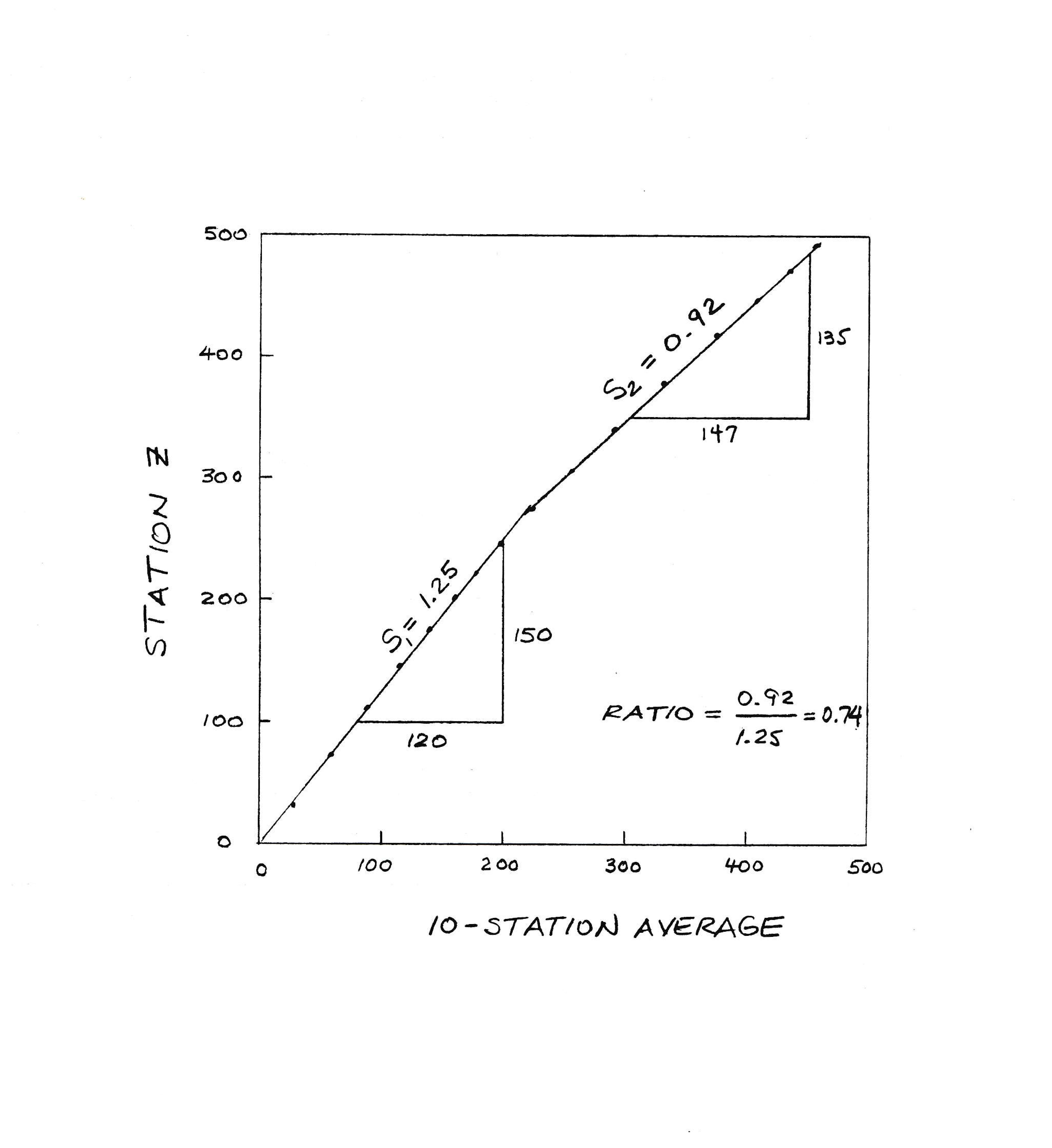
The computations are shown in Fig. M-2-12 and in the following table.
| Year |
Station Z
(mm) |
10-station
average
(mm) |
Σ Z |
Σ 10-station
average |
Station Z
corrected
(mm) |
| 1972 |
35 |
28 |
35 |
28 |
25.9 |
| 1973 |
37 |
29 |
72 |
57 |
27.4 |
| 1974 |
39 |
31 |
111 |
88 |
28.9 |
| 1975 |
35 |
27 |
146 |
115 |
25.9 |
| 1976 |
30 |
25 |
176 |
140 |
22.2 |
| 1977 |
25 |
21 |
201 |
161 |
18.5 |
| 1978 |
20 |
17 |
221 |
178 |
14.8 |
| 1979 |
24 |
21 |
245 |
199 |
17.8 |
| 1980 |
30 |
26 |
275 |
225 |
22.2 |
| 1981 |
31 |
31 |
306 |
256 |
|
| 1982 |
35 |
36 |
341 |
292 |
|
| 1983 |
38 |
39 |
379 |
331 |
|
| 1984 |
40 |
44 |
419 |
375 |
|
| 1985 |
28 |
32 |
447 |
407 |
|
| 1986 |
25 |
30 |
472 |
437 |
|
| 1987 |
21 |
23 |
493 |
460 |
|
|
|
Fig. M-2-12 Double mass analysis for Problem 2-12.
|
After 1980, there is a break in the slope of the double-mass curve, as
shown in Fig. M-2-12. The slope of the double-mass curve up to 1980 is
1.25; the slope after 1980 is 0.92. The ratio of slopes after and
before the break is 0.92/1.25 = 0.74. To reflect the change in trend,
the records of station Z prior to the break are corrected by
multiplying by 0.74, as shown in the last column. ANSWER.
|
Calculate the interception
loss for a storm lasting 30 min, with interception storage 0.3 mm, ratio of evaporating
foliage surface to its horizontal projection K = 1.3, and evaporation rate E = 0.4 mm/h.
|
Using Eq. 2-12, the interception loss is: L = 0.3 mm + (1.3 × 0.4 mm/h
× 30 min × 1 h / 60 min) = 0.56 mm. ANSWER.
|
Show that F = (fo - fc)/k,
in which F is the total infiltration depth above the
f = fc line, Eq. 2-13.
|
Since F is the total infiltration depth above the f = fc line:
∞
F = ∫(fo - fc ) e-kt dt
0
Therefore:
∞
F = [ - (fo - fc ) / k ] [e-kt ] = (fo- fc)/k. ANSWER.
0
|
Fit a Horton infiltration formula to the following
measurements:
Time
(h) | f
(mm/h) |
| 1 | 2.35 |
| 3 | 1.27 |
| ∞ | 1.00 |
|
Since at t = ∞, the final infiltration rate is 1 mm/h, then: fc = 1
mm/h. Therefore, from Eq. 2-13:
2.35 = 1 + (fo - 1) e-k; and
1.27 = 1 + (fo - 1) e-3k
Then: fc = 1 mm/h; fo = 4.019 mm/h; and k = 0.8047 h-1. ANSWER.
|
Given the
following measurements, determine the parameters of the Philip infiltration equation.
Time
(h) | f
(mm/h) |
| 2 | 1.7 |
| 4 | 1.5 |
|
Using Eq. 2-15:
1.7 = (1/2) s (2)-1/2 + A
1.5 = (1/2) s (4)-1/2 + A
Solving for s and A: s = 1.932 h1/2; A = 1.017 mm/h. ANSWER.
|
The following rainfall distribution was measured
during a 12-h storm:
|
Time (h) | 0-2 | 2-4 | 4-6 | 6-8 | 8-10 | 10-12 |
| Rainfall intensity (cm/h) |
1.0 | 2.0 | 4.0 | 3.0 | 0.5 | 1.5 |
Runoff depth was 16 cm. Calculate the φ-index for this storm.
|
Try several likely values for φ. For instance, assume φ between 0.5
and 1.0 cm/h. Therefore:
2 × (1 - φ) + 2 × (2 - φ) + 2 × (4 - φ)
+ 2 × (3 - φ) + 2 × (1.5 - φ) = 16.
Solving for φ: φ = 0.7 cm/h.
Therefore, the assumption of φ being between 0.5 and 1.0 cm/h was
correct. ANSWER.
|
Using the data of Problem 2-17, calculate the W-index, assuming the sum of
interception loss and depth of surface storage is S = 1 cm.
|
Use Eq. 2-19, with P = 240 mm; Q = 160 mm; S = 10 mm. Assume that tf,
the total time during which rainfall intensity is greater than W, is
tf = 10 h.
Therefore: W = (240 - 160 - 10)/10 = 7 mm/h.
With W = 7 mm/h, it is verified that the assumption tf = 10 h was correct. ANSWER.
|
A certain catchment has a depression storage capacity of Sd = 2 mm. Calculate the equivalent depth of depression
storage for the following values of precipitation excess: (a) 1 mm, (b) 5 mm, and (c) 20 mm.
|
Since k = 1/Sd = 0.5 mm-1, then, using Eq. 2-20:
a) For Pe = 1 mm: Vs = 2 (1 - e -0.5 (1)) = 0.78 mm. ANSWER.
b) For Pe = 5 mm: Vs = 2 (1 - e-0.5 (5)) = 1.83 mm. ANSWER.
c) For Pe = 20 mm: Vs = 2 (1 e -0.5 (20)) = 1.99 nm. ANSWER.
It is seen that surface storage fills up with precipitation excess,
exponentially reaching the limit Sd.
|
-
Use the Meyer equation to calculate monthly evaporation for a large lake, given the following data:
month of July, mean monthly air temperature 70°F, mean monthly relative humidity 60%,
monthly mean wind speed at 25-ft height, 20 mi/h.
|
Since monthly evaporation is required, use Eq. 2-28a. The saturation
vapor pressure for the given temperature (70°F) is obtained from Table
A-2: 0.739 in. Hg. The (partial) vapor pressure of the air is: 0.739
× (RH/100) = 0.739 × (60/100) = 0.4434 in. Hg. Since this is a large
lake, use C = 11. Using Eq. 2-28a: E = 11 × [0.739 - 0.4434] × [1 +
(20/10)] = 9.75 in./mo. ANSWER.
|
Derive the Penman equation (Eq. 2-35).
|
A balance of the incoming energy and energy expenditure leads to:
|
Qs (1 - A ) - Qb + Qa = Qh + Qe + Qt | (1) |
Assuming Qa = 0 and Qt = 0, the energy balance reduces to:
|
Qs (1 - A) - Qb = Qh + Qe | (2) |
The left-hand side of Eq. 2 is the net solar radiation Qn; the
right-hand side can be expressed in terms of Bowen's ratio. Therefore:
Converting to evaporation rate units:
For p = 1000 millibars, the Bowen ratio (Eq. 2-24) is:
|
B = γ(Ts - Ta) / (es - ea) | (5) |
The saturation vapor-pressure gradient (Eq. 2-33) is:
|
Δ = (es - eo) / (Ts - Ta) | (6) |
The ratio of mass transfer evaporation (assuming that the temperature
of water surface and overlying air are equal) to actual evaporation
(Eq. 2-34) is:
|
Ea / E = (eo - ea) / (es - ea) | (7) |
From Eqs. 4 and 5:
|
En / E = 1 + γ(Ts - Ta) / (es - ea) | (8) |
Substituting Eq. 6 in 8:
|
En / E = 1 + (γ/Δ)(es - eo) / (es - ea) | (9) |
|
En / E = 1 + (γ/Δ) [(es - ea) - (eo - ea)] / (es - ea) | (10) |
Substituting Eq. 7 in Eq. 10:
|
En / E = 1 + (γ/Δ) [1 - (Ea / E)] | (11) |
Solving for E:
|
E = (ΔEn + γEa) / (Δ + γ) | (12) |
which is the Penman equation (Eq. 2-35). ANSWER.
|
Use the Penman method to calculate the evaporation rate for the following atmospheric
conditions: air temperature, 25°C; net radiation, 578 cal/cm2/d, wind speed at 2-m above the
surface, v2 = 150 km/d; relative humidity, 50%.
|
From Table 2-4, for Ta = 25�C, α = 2.86.
From Table A-1 (Appendix A), for Ta = 25�C, the heat of vaporization
is: H = 583.2 cal/g, and the density ρ = 0.99705 g/cm3. The net
radiation in evaporation units (solving from Eq. 2-23) is:
En = (578 cal/cm2/d) / (0.99705 g/cm3 × 583.2 cal/g) = 0.994 cm/d.
The saturation vapor pressure at the air temperature (Table A-1) is:
eo = 31.67 mb.
Using the Dunne formula (Eq. 2-38), the mass-transfer
evaporation is:
Ea = [0.013 + (0.00016 × 150)] × (31.67) × [(100 -
50)/100] = 0.586 cm/d.
Using Eq. 2-38: E = [(2.86 × 0.994) + 0.586] /
(2.86 + 1) = 0.89 cm/d. ANSWER.
|
Use the Penman method (together with
the Meyer equation) to calculate the evaporation rate (in inches per day) for the following
atmospheric conditions: air temperature, 70°F, water surface temperature, 50°F, daily mean wind
speed at 25-ft height, W = 15 mi/h, relative humidity 30%, net radiation, Qn = 15 Btu/ in.2/ d.
Assume a large lake to use Eq. 2-27 (b).
|
The saturation vapor pressure at the water surface temperature (Table
A-2, Appendix A) is: es= 0.362 in. Hg. The vapor pressure of the air
is equal to the saturation vapor pressure at the air temperature (Table
A-2) (0.739 in. Hg.) multiplied by the relative humidity in percentage
and divided by 100: ea = 0.739 × (30 / 100) = 0.2217 in. Hg. For a large
lake, C = 0.36. Using the Meyer equation for daily evaporation (Eq.
2-27b), the mass-transfer evaporation rate is:
Ea = 0.36 × (0.362 - 0.2217) × [1 + (15/10)] = 0.126 in./d.
The net radiation in evaporation rate units (solving from Eq. 2-23) is:
En = (15 Btu/in.2/day × 1728 in.3/ft3) / (62.3 lb/ft3 × 1054 Btu/lb)
En = 0.395 in./d.
From Table 2-4, for Ta = 70�F (21.11�C), α = 2.34 (by linear interpolation).
Using Eq. 2-37:
E = [(2.34 × 0.395) + 0.126] / (2.34 + 1) = 0.314 in./d. ANSWER.
|
Use the Blaney-Criddle method (with corrections
due to Doorenbos and Pruitt) to calculate reference crop evapotranspiration during the month of
July for a geographic location at 40°N, with mean daily temperature of 25°C. Assume high actual
insolation time, 70% minimum relative humidity, and 1 m/s daytime wind speed.
|
From Table A-3 (Appendix A), for 40�N, during the month of July: p =
0.33.
Using Eq. 2-41: f = 0.33 × [(0.46 × 25) + 8.13] = 6.48 mm/d.
With Fig. 2-16, the value of f is corrected for the effects of high
actual insolation time, 70% minimum relative humidity (high), and 1 m/s
diurnal wind speed (low) (a = -2.15, b = 1.14, graph III, curve 1):
ETo = -2.15 + (1.14 × 6.48) = 5.24 mm/d.
For the month of July (31 days), the reference crop evapotranspiration is:
ETo = 5.24 × 31 = 162 mm. ANSWER.
|
Use the
Thornthwaite method to calculate the potential evapotranspiration during the month of May for a
geographic location at 35°N, with the following mean monthly temperatures, in degrees Celsius.
|
Jan | Feb | Mar | Apr | May |
Jun | Jul | Aug | Sep | Oct | Nov | Dec |
| 6 |
8 | 10 | 12 | 15 | 20 | 25 |
20 | 16 | 12 | 10 | 8 |
|
Using Eq. 2-43, the monthly heat indexes are:
|
Jan | Feb | Mar | Apr | May |
Jun | Jul | Aug | Sep | Oct | Nov | Dec |
1.32 | 2.04 | 2.86 | 3.76 | 5.28 | 8.16 |
11.43 | 8.16 | 5.82 | 3.76 | 2.86 | 2.04 |
The temperature efficiency index J is the sum of the monthly heat
indexes I: J = 57.49.
Using Eq. 2-45: c = 1.396.
Using Eq. 2-44 for
the month of May: PET (0) = 6.10 cm/mo.
Using Table A-4 (Appendix A):
PET = 1.17 × 6.10 = 7.14 cm during the month of May. ANSWER.
|
Use the Priestley and Taylor formula to calculate the potential evapotranspiration for a site with
air temperature of 15°C and net radiation of 560 cal/cm2/d.
|
From Table A-1 (Appendix A), for T = 15�C, the heat of vaporization H is:
H = 588.9 cal/g, and the density of water is ρ = 0.9991 g/cm3.
From Table 2-6: α = 1.654.
Using Eq. 2-47(b):
PET = 1.26 × 1.654 × [(560 cal/cm2/d) / ( 0.9991 g/cm3
× 588.9 cal/g )] / (1.654 + 1) = 0.747 cm/d. ANSWER.
|
The following data have been
obtained by planimetering a 135-km2 catchment:
Elevation
(m) | Subarea above
indicated elevation
(km2) |
| 1010 | 135 |
| 1020 | 85 |
| 1030 | 65 |
| 1040 | 30 |
| 1050 | 12 |
| 1060 | 4 |
| 1070 | 0 |
Calculate a hypsometric curve for
this catchment.
|
The minimum elevation is: Emin = 1010; the maximum elevation is: Emax = 1070.
The difference in elevation is: ΔE = 1070 - 1010 = 60.
The catchment area is: Ac = 135 km2. The abscissas and ordinates of the hypsometric curve are shown below.
Elevation
Ei
(m) |
Subarea
Ai
(km2) |
Abscissas
(Ai / Ac) ×100
(percentage) |
Ordinates
[(Ei - Emin) / ΔE] ×100
(percentage) |
| 1010 |
135 |
100.0 |
0.0 |
| 1020 |
85 |
62.9 |
16.6 |
| 1030 |
65 |
48.1 |
33.3 |
| 1040 |
30 |
22.2 |
50.0 |
| 1050 |
12 |
8.9 |
66.7 |
| 1060 |
4 |
2.9 |
83.3 |
| 1070 |
0 |
0.0 |
100.0 |
|
|
- Derive the formula for the compactness ratio Kc (Eq. 2-51).
|
Assume the area and perimeter of the catchment to be A and P, respectively.
Assume the area and perimeter of the equivalent circle to be Ao and Po, respectively.
Ao = A
Ao = π r 2 ; From which: r = (Ao / π) 1/2
Po = 2 π r
Po = 2 π (Ao / π)1/2 = 2 ( π Ao)1/2
Compactness ratio:
Kc = P / Po = P / [ 2 (π Ao)1/2]
Kc = P / [ 2 (πA)1/2] = 0.282 P / A1/2. ANSWER.
|
Given the following longitudinal profile
of a river channel, calculate the following slopes: (a) S1, (b) S2, and (c) S3.
|
Distance (km) | 0 | 50 | 100 | 150 |
200 | 250 | 300 |
| Elevation (m) |
10 | 30 | 60 | 100 |
150 | 220 | 350 |
|
(a) The S1 slope is: S1 = (350 - 10) / 300,000 = 0.001133. ANSWER.
(b) Using the trapezoidal rule, the area below the longitudinal profile
and above Elevation 10 is: [340 + 2 × (210 + 140 + 90 + 50 + 20)] ×
(50,000/2) = 34,000,000 m2.
From Fig. 2-41: Y (300,000/2) =
34,000,000. Therefore: Y = 226.67 m. The S2 slope is: S2 =
Y/300,000 = 0.000756. ANSWER.
(c) The individual subreaches are all of length Li = 50 km. Using
Eq. 2-52, the S3 slope is calculated as shown in the following table:
Distance
(km) |
Elevation
(m) |
Slope Si |
Li / Si1/2 |
| 0 |
10 |
- |
- |
| 50 |
30 |
0.0004 |
2500 |
| 100 |
60 |
0.0006 |
2041 |
| 150 |
100 |
0.0008 |
1768 |
| 200 |
150 |
0.0010 |
1581 |
| 250 |
220 |
0.0014 |
1336 |
| 300 |
350 |
0.0026 |
981 |
| Sum |
|
|
10,207 |
|
|
Fig. M-2-29 Calculation of slopes S1, S2 and S3 .
|
Using Eq. 2-52: S3 = (300/10,207)2 = 0.000864. The three slopes
are plotted in Fig. M-2-29. ANSWER.
|
The bottom of a certain 100-km reach of a river can be
described by the following longitudinal
profile:
y = 100 e -0.00001 x
in which y = elevation with reference to an arbitrary datum,
in meters; and x = horizontal distance measured from upstream end of the reach, in meters. Calculate
the S2 slope.
|
At x = 0 km, elevation y = 100 m. At x = L = 100,000 m, elevation y =
36.78794 m.
From Fig. 2-41, the area comprised between elevation
36.78794 and the longitudinal profile is: A = YL/2.
Therefore, the S2 slope is: S2 = Y/L = 2A/L2.
The total area At below the longitudinal profile is obtained by
integration:
100,000
At = ∫ y dx = 6,321,206 m2
0
The area comprised between elevation 0 and elevation 36.78794 m is:
Ab = 36.78794 × 100,000 = 3,678,794 m2. Therefore, the area A is:
A = At - Ab = 2,642,412 m2. And: S2 = 2A/L2 = 0.0005285. ANSWER.
|
Given the following 14-d record of daily precipitation, calculate the
antecedent precipitation index API. Assume the starting value of the index to be equal to 0 and
the recession constant K = 0.85.
|
| Day | Precipitation
(cm) |
| 1 | 0.0 |
| 2 | 0.1 |
| 3 | 0.3 |
| 4 | 0.4 |
| 5 | 0.2 |
|
| Day | Precipitation
(cm) |
| 6 | 0.0 |
| 7 | 0.0 |
| 8 | 0.7 |
| 9 | 0.8 |
| 10 | 0.9 |
|
| Day | Precipitation
(cm) |
| 11 | 1.2 |
| 12 | 0.5 |
| 13 | 0.0 |
| 14 | 0.0 |
| | |
|
|
Equation 2-56 is used to calculate the antecedent precipitation index,
with the daily precipitation added to the index. The calculations are
shown in the following table.
| Day |
Precipitation
(cm) |
Antecedent Precipitation Index API
(cm) |
| 1 |
0.0 |
0.000 |
| 2 |
0.1 |
0.100 |
| 3 |
0.3 |
0.385 |
| 4 |
0.4 |
0.727 |
| 5 |
0.2 |
0.818 |
| 6 |
0.0 |
0.695 |
| 7 |
0.0 |
0.591 |
| 8 |
0.7 |
1.202 |
| 9 |
0.8 |
1.822 |
| 10 |
0.9 |
2.449 |
| 11 |
1.2 |
3.281 |
| 12 |
0.5 |
3.289 |
| 13 |
0.0 |
2.795 |
| 14 |
0.0 |
2.376 |
|
|
A 35-ha catchment
experiences 5 cm of precipitation, uniformly distributed in 2 h. If the time of concentration
is 1 h, what is the maximum possible flow rate at the catchment outlet?
|
The average precipitation intensity is 25 mm/h. Since the time of
concentration is 1 h and the rainfall duration is 2 h, the catchment
flow is superconcentrated.
The maximum possible flow rate is obtained by assuming zero hydrologic
abstractions (Qe = IA):
Qe = (25 mm/h × 35 ha × 10,000 m2/ha) / (3600 s/h × 1000 mm/m)
Qe = 2.43 m3/s. ANSWER.
|
Calculate hourly
ordinates of a gamma hydrograph with the following characteristics: peak flow, 1000 m3/s;
baseflow, 0 m3/s; time-to-peak, 3 h; and time-to-centroid, 6 h.
|
With Qp = 1000 m3/s; Qb = 0; tp = 3 h; andtg = 6 h; and Eq. 2-64:
Q = 1000 (t / 3) e1 - (t / 3)
The hourly ordinates are shown in the following table.
|
t
(h) | Q
(m3/s) |
| 1 | 649 |
| 2 | 930 |
| 3 | 1000 |
| 4 | 955 |
| 5 | 856 |
| 6 | 736 |
|
t
(h) | Q
(m3/s) |
| 7 | 615 |
| 8 | 504 |
| 9 | 406 |
| 10 | 323 |
| 11 | 255 |
| 12 | 199 |
|
t
(h) | Q
(m3/s) |
| 13 | 155 |
| 14 | 119 |
| 15 | 92 |
| 16 | 70 |
| 17 | 53 |
| 18 | 40 |
|
The following data
have been measured in a river: mean velocity V = 1.8 m/s, hydraulic radius R = 3.2 m, channel
slope S = 0.0005. Calculate the Manning and Chezy coefficients.
|
Using Eq. 2-65:
n = R 2/3 S 1/2 / V = (3.2) 2/3 (0.0005)1/2 / 1.8 = 0.027. ANSWER.
Using Eq. 2-66:
C = V / (R 1/2 S 1/2) = 1.8 / [(3.2)1/2 ×(0.0005) 1/2] = 45 ml/2/s. ANSWER.
|
The Chezy coefficient
for a wide channel is C = 49 m1/2/s and the bottom slope is
S = 0.00037. What is the Froude number of
the uniform (i.e., steady equilibrium) flow?
|
With C = 49 m1/2/s, f = g / C 2 = 9.81/(49)2 = 0.004086.
From Eq. 2-68: F = (0.00037/0.004086)1/2 = 0.30. ANSWER.
|
The flow
duration characteristics of a
certain stream can be expressed as follows:
Q = ( 950 /T ) + 10
in which Q = discharge in cubic
meters per second, and T = percent time, restricted to the range 1-100%. What flow can be
expected to be exceeded: (a) 90% of the time, (b) 95% of the time, and (c) 100% of the time?
|
(a) Q = (950/90) + 10 = 20.5 m3/s. ANSWER.
(b) Q = (950/95) + 10 = 20.0 m3/s. ANSWER.
(c) Q = (950/100) + 10 = 19.5 m3/s. ANSWER.
|
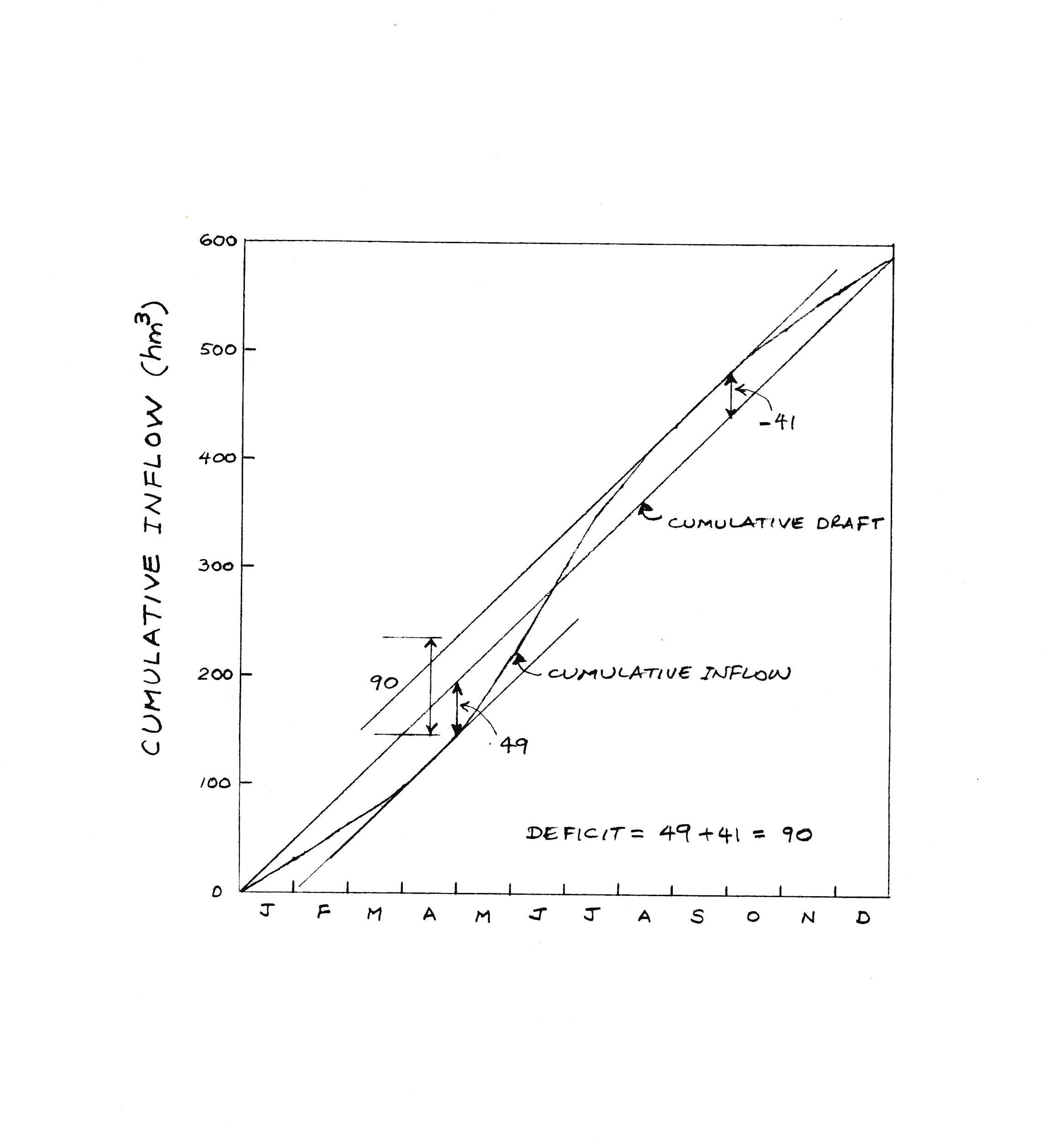
A reservoir has the following average monthly inflows, in cubic hectometers (million of cubic meters):
|
Jan | Feb | Mar | Apr | May |
Jun | Jul | Aug | Sep | Oct | Nov | Dec |
| 30 | 34 | 35 | 48 | 72 | 85 |
72 | 55 | 51 | 40 | 34 | 32 |
Determine the reservoir
storage volume required to release a constant draft rate throughout the year.
|
The calculations of the flow-mass curve are shown in the following table.
| (1) | (2) | (3) | (4) | (5) |
Month |
Inflow
(hm3) |
Cumulative
inflow
(hm3) |
Cumulative
draft
(hm3) |
Deficit
(hm3) |
| Jan |
30 |
30 |
49 |
19 |
| Feb |
34 |
64 |
98 |
34 |
| Mar |
35 |
99 |
147 |
48 |
| Apr |
38 |
147 |
196 |
49 |
| May |
72 |
219 |
245 |
26 |
| Jun |
85 |
304 |
294 |
-10 |
| July |
72 |
376 |
343 |
-33 |
| Aug |
55 |
431 |
392 |
-39 |
| Sep |
51 |
482 |
441 |
-41 |
| Oct |
40 |
522 |
490 |
-32 |
| Nov |
34 |
556 |
539 |
-17 |
| Dec |
32 |
588 |
588 |
0 |
|
The total cumulative inflow during the year is the last value of Col.
3: 588 hm3. This value is divided by 12 to obtain the constant draft
rate: 49 hm3/mo. The cumulative draft shown in Col. 4 is obtained by
adding the (constant) monthly draft rates. The deficit is equal to the
inflow (Col. 4) minus the draft (Col. 5). The required reservoir
storage is the sum of the maximum positive and negative deficits:
49 + 41 = 90 hm3. The graphical solution is shown in Fig. M-2-37. ANSWER.
|
Fig. M-2-37 Flow-mass curve.
|
|
The
analysis of 43 y of runoff data at a reservoir site in a large river has led to the following:
mean annual runoff volume, 24 km3; standard deviation, 7 km3. What is the reservoir storage
volume required to guarantee a constant release rate equal to the mean of the data?
|
Using Eq. 2-71: R = 7 km3 × (43/2)0.73 = 66 km3. ANSWER.
|
Calculate the peak discharge for a 1000-mi2 drainage area using the Creager
formula (Eq. 2-73) with (a) C = 30, and (b) C = 100.
|
a) Using Eq. 2-73, with C = 30:
qp = 116 ft3/s, and Qp = 116,000 ft3/s. ANSWER.
(b) Using Eq. 2-73, with C = 100:
qp = 387 ft3/s, and Qp = 387,000 ft3/s. ANSWER.
|
| http://enghydro.sdsu.edu |
|
200723 14:01 |
|
|