Generalized conceptual modeling
of dimensionless overland flow hydrographs


Victor M. Ponce
O. I. Cordero-Braña
and
S. Y. Hasenin


Online version 2016

[Original version 1997]


ABSTRACT

The rising and recession limbs of conceptual dimensionless overland flow hydrographs are calculated for specific values of the rating exponent in the range 1 ≤ m ≤ 3, including a linear reservoir (m = 1); 100% turbulent Cheazy friction (m = 3/2); 100% turbulent Manning friction (m = 5/3); 67% turbulent Chezy (or 75% turbulent Manning) (m = 2); and 100% laminar flow (m = 3). These conceptual overland flow hydrographs show finite amounts of diffusion, increasing with decreasing rating exponent, unlike the kinematic wave hydrograph, which is nondiffusive.

Keywords: Dimensionless; Overland flow; Hydrographs; Conceptual modeling.


1.  INTRODUCTION

The calculation of overland flow hydrographs is well established in flood hydrology. Early approaches had a distinct conceptual basis (Horton, 1938,1945; lzzard, 1944,1946), while more recent approaches, among them the kinematic wave, have relied on the physics of the phenomena (Wooding, 1965; Woolhiser and Liggett, 1967). The kinematic wave lacks diffusion and, therefore, is not suited for overland flow over mild slopes, where diffusion plays a major role. On the other hand, the conceptual model has an intrinsic diffusion capability, which is underscored by the fact that its reference time-to-equilibrium is twice that of the kinematic wave (Ponce, 1989).

A conceptual model of dimensionless overland flow hydrographs is presented here. The procedure generalizes the classical Horton-Izzard approach for a wide range of rating exponents, including m = 3/2 and 5/3, which, to our knowledge, have not been previously calculated. The rising and recession limbs of dimensionless overland flow hydrographs are calculated for the following values of the rating exponent: (1) linear reservoir, m = 1, describing a condition where the overland flow velocity is sensibly constant (Houton, 1938); (2) 100% turbulent Chezy friction, m = 3/2; (3) 100% turbulent Manning friction, m = 5/3; (4) 67% turbulent Chezy friction (equivalent to 75% turbulent Manning), m = 2; and (5) 100% laminar flow, m = 3.


2.  THE CONCEPTUAL MODEL

Runoff in the overland flow plane is described by the differential equation of storage:

               dS           
I - O  =  _____
               dt     
(1)

in which I = inflow, O = outflow, and dS / dt = rate of change of storage in the plane.

A mass balance leads to the equilibrium outflow:


qe = iL

(2)

in which i = rainfall excess, and L = length of the plane. For the rising limb, I = iL, and O = q, from which:

                dS           
iL - q  =  _____
                dt     
(3)

For the receding limb, I = 0, and O = q, from which:

           dS           
-q  =  _____
           dt     
(4)

The Horton-Izzard model is based on the discharge-storage rating:


q = a S m

(5)

in which a and m are coefficient and exponent, respectively. Equation 5 is assumed to be applicable for any discharge, including that at equilibrium. Additionally, the equilibrium storage is equal to:

            qe te           
Se  =  _______
              2  
(6)

in which te = reference time-to-equilibrium. Because of runoff diffusion, the equilibrium outflow is approached asymptotically, i.e. qqe as t → ∞. Thus, the reference time-to-equilibrium is less than the actual time-to-equilibrium, which approaches infinity. For the rising limb, the generalized conceptual model is:

                           dS           
a Sem - a Sm =  _____
                           dt     
(7)

The solution of Eq. 7 is (Dooge, 1973; Ponce, 1989):

          1          1
t *  = ____ ______ d ( q * 1/m )
          2      1 - q *
(8)

in which t * = t / te, with t = the accumulated time from the start of rising, and te = the reference time-to-equilibrium, and q * = q / qe, with q = the outflow at time t, and qe = the equilibrium outflow.

For the receding limb, the generalized conceptual model is:

                  dS           
- a Sm  =  _____
                  dt     
(9)

The solution for the receding limb depends on whether the rising limb has reached equilibrium or not. First, assuming that the rising limb is at equilibrium, the solution of Eq. 9 is (Dooge, 1973):

            1         1
t *  = - ___  _____ d ( q * 1/m )
            2        q *
(10)

in which t * = t / te, with t = the accumulated time from the start of recession, and t * = the reference time-to-equilibrium (of the rising limb); and q * = q /qe, with q = the outflow at time t, and qe = the outflow at the start of recession, i.e. the equilibrium outflow.

Assuming that the peak outflow at the end of the rising limb is qp, less than the equilibrium outflow (qe), the solution of Eq. 9 is:

            1        qp                            1
t *  = - ___ ( _____ ) (1 - m) / m    ____ d ( q * 1/m )
            2        qe                          q *
(11)

in which t * is the same as in Eq. 10, but now q * = q /qp.

Equation 8 is evaluated herein for values of m equal to 1, 3/2, 5/3, 2 and 3.

1.  m = 1

                1           
    t *  = - ___ ln ( 1 - q * )
                2    
(12)

2.  m = 3/2

                  1                          1                          1
    t *  = - ______ { arctan ( ______ ) - arctan [ ______ ( 1 + 2 q *1/3 ) ] }
               (3)1/2                   (3)1/2                    (3)1/2

           1                                   1
    - ( ___ ) ln ( 1 - q *1/3 ) + ( ___ ) ln ( 1 + q *1/3 + q *2/3 )
           3                                   6

(13)

3.  m = 5/3

    t * = - 0.3 ln ( 1 - q *1/5 ) + 0.3 cos ( 0.6 π ) ln [1 + q *2/5 + 2 q *1/5 cos ( 0.2 π )]

    + 0.3 cos (1.8 π ) ln [ 1 + q *2/5 + 2 q *1/5 cos (0.6 π )]

                                                  q *1/5 + cos (0.2 π)
    + 0.6 sin (0.6 π ) { arctan [ _____________________] - 0.3 π }
                                                        sin (0.2 π)

                                                  q *1/5 + cos (0.6 π)
    + 0.6 sin (1.8 π ) { arctan [ _____________________] + 0.1 π }
                                                        sin (0.6 π)

(14)

4.  m = 2

              1            1 + q *1/2
    t * = ____ ln ( ____________)
              4            1 - q *1/2
(15)

5.  m = 3

              1            1 + q *1/3 + q *2/3
    t * = ____ ln [ ____________________]
              4                ( q *1/3 - 1 ) 2

             1              π                           1
    - __________ { _____ + arctan [ - _______ (1 + 2 q *1/3 ) ]}
        2 (3)1/2          6                        (3)1/2

(16)

Following Dooge (1973), the solution of Eq. 10 for m = 1 and m > 1 is:

1.  m = 1

                1           
    t *  = - ___ ln q *
                2   
(17)

2.  m > 1

                      1           
    t *  = - ____________ ( q *(1 - m) / m - 1 )
                2 ( m - 1 )   
(18)

where q * = 1 at t * = 0, i.e., the outflow is at equilibrium at the start of the recession.

The solution of Eq. 11 parallels that of Eq. 10, but in this case q * = q /qp, and t * is affected by an appropriate dimensionless outflow factor (compare Eq. 10 and 11).

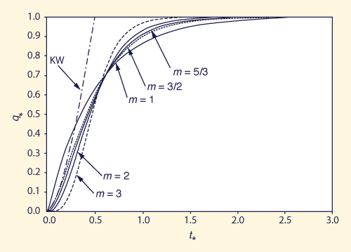
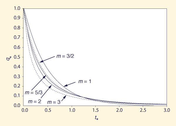
Figures 1 and 2 show the rising and recession dimensionless overland flow hydrographs calculated with Eqs. 12-16 and Eqs. 17 and 18, respectively. Also included in Fig. 1 is the rising limb of the kinematic wave overland flow model, for m = 3/2, expressed in terms of t * for comparison (Ponce, 1989):

           1           
t *  =  ___ q *1/m
           2      
(19)

As Fig. 1 shows, the conceptual models of overland flow have asymptotic solutions, and am therefore, able to simulate runoff diffusion. Figure 1 also shows that diffusion is greatest for m = 1, the case of a linear reservoir. Within the range 1 ≤ m ≤ 3, diffusion is smallest for m = 3.

Dimensionless relative wave celerity vs dimensionless wavenumber

Fig. 1  Rising limb of cenceptual dimensionless overland flow hydrograph
for selected values of the rating exponent m.

Dimensionless relative wave celerity vs dimensionless wavenumber

Fig. 2  Receding limb of conceptual overland flow hydrograph
for selected values of the rating exponent m.


3.  SUMMARY

We calculate conceptual dimensionless overland flow hydrographs for five rating exponents in the range m = 1 (linear reservoir) to m = 3 (laminar flow). The resulting hydrographs show that it is possible to simulate varying amounts of diffusion with the conceptual overland flow models, unlike the kinematic wave model, which is nondiffusive.


REFERENCES

Dooge, J. C. I. 1973. Linear theory of hydrologic systems. Technical Bulletin 1468, US Department of Agriculture, Washington, DC, pp. 327.

Horton, R. E. 1938. The interpretation and application of runoff plot experiments with reference to soil erosion problems. Proc. Soil Sci. Soc. Am. 3, 340-349.

Horton, R. E. 1945. Erosional development of streams and their drainage basins: Hydrophysical approach to quantitative geomorphology. Bull. Geol. Soc. Am. 56, 275-370.

Izzard, C. F. 1944. The surface profile of overland flow. Trans. Am. Geophys. Union 25 (6), 959-968.

Izzard, C. F. 1946. Hydraulics of runoff from developed surfaces. Proc. Highway Res. Board, Washington, DC 26, 129-146.

Ponce, V. M. 1989. Engineering Hydrology, Principles and Practices. Prentice Hall, Englewood Cliffs, NJ.

Wooding, R. A. 1965. A hydraulic model for the catchment-stream problem. J. Hydrol. 3, 254-267.

Woolhiser, D. A. and J. A. Liggett, 1967. Unsteady one-dimensional flow over a plane - the rising hydrograph. Water Resour. Res. 3(3), 753-771.


211230

Documents in Portable Document Format (PDF) require Adobe Acrobat Reader 5.0 or higher to view; download Adobe Acrobat Reader.