skip to main content

ABSTRACT Gradually varied flow water-surface profiles are expressed in terms of the critical slope Sc. In this way, the flow-depth gradient dy/dx is shown to be strictly limited to values outside the range encompassed by Sc and So, in which So is the bed slope. This approach improves and completes the definition of flow-depth-gradient ranges in the analysis of water surface profiles. Online calculators are provided to round up the experience.

Q 2 T F 2  =  _______               g A 3 (3)

Combining Equations 2 and 3 leads to:

Sf  =  (P / T ) (g / C 2) F 2 (4)

At normal critical flow, F = 1, and the friction slope at critical state, i.e., the critical slope, is:

Sc  = (Pc / Tc ) (g / C 2) (5)

Combining Equations 1, 4, and 5:

dy          So - Sc F 2 ___  =  ___________  dx             1 - F 2 (6) which is strictly valid for the following condition:  P /T = Pc /Tc . This latter condition is generally satisfied in a hydraulically wide channel, for which T is asymptotically equal to P. For ease of expression, the flow-depth gradient is renamed Sy = dy/dx. Solving for Froude number from Equation 6:                So - Sy F 2  =   _________                Sc - Sy (7) Since F 2 > 0, the flow-depth gradient must satisfy the following inequalities: So ≥ Sy ≤ Sc (8) So ≤ Sy ≥ Sc (9) which effectively limits the flow-depth gradient to values outside the range encompassed by So and Sc. Furthermore, Equation 6 can be alternately expressed as follows:  Sy          ( So / Sc ) - F 2 ___  =  ______________  Sc                1 - F 2 (10) Equation 10 is the GVF equation in terms of bed slope So , critical slope Sc , and Froude number F. The bed slope could be positive (steep, critical, or mild), zero (horizontal), or negative (adverse). The critical slope (Equation 5) and Froude number squared (Equation 3) are always positive. 3.  CLASSIFICATION OF WATER-SURFACE PROFILES Equation 10 is used to develop a classification of water-surface profiles based solely on the three dimensionless parameters: Sy /Sc , So /Sc , and F. 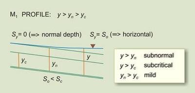For the sake of completeness, subcritical flow is defined as that for which the flow depth is greater than the critical depth (F 2 < 1) (Chow 1959; Henderson 1966). Paralleling this widely accepted definition, subnormal flow is defined as that for which the flow depth is greater than the normal depth [F 2 < So /Sc ]. Supernormal flow is defined as that for which the flow depth is smaller than the normal depth [F 2 > So /Sc ] (USDA SCS 1971). Table 1 shows the four (4) classes of water-surface profiles and the twelve (12) possible profiles. Table 1.  Possible classes and types of water-surface profiles. CLASS 1:  SUBCRITICAL/SUBNORMAL Steep:  S1 Critical:  C1 Mild:  M1 CLASS 2A:  SUPERCRITICAL/SUBNORMAL Steep:  S2 CLASS 2B:  SUBCRITICAL/SUPERNORMAL Mild:  M2 Horizontal:  H2 Adverse:  A2 CLASS 3:  SUPERCRITICAL/SUPERNORMAL Steep:  S3 Critical:  C3 Mild:  M3 Horizontal:  H3 Adverse:  A3 A summary of the twelve possible water-surfaces profiles is shown in Table 2. The classification follows directly from the governing equation (Equation 10). It is seen that the general class of profile (Class 1, 2A, 2B, or 3) determines the sign of Sy /Sc (Column 2) and, thus, the classification of either backwater or drawdown (Column 3). Also, the general class of profile determines the feasible range of So /Sc (Column 4) and, thus, the existence of specific profiles types (Steep, Critical, Mild, Horizontal, or Adverse) within each general type. Note that not all combinations of Sy /Sc and So /Sc are feasible. Unlike the description available in standard references (Chow 1959; Henderson 1966), the flow-depth gradient ranges (Table 2, Columns 7 and 8) are now complete for all twelve water-surfaces profiles. Significantly, the flow-depth gradient Sy is shown to be outside the range encompassed by Sc and So . 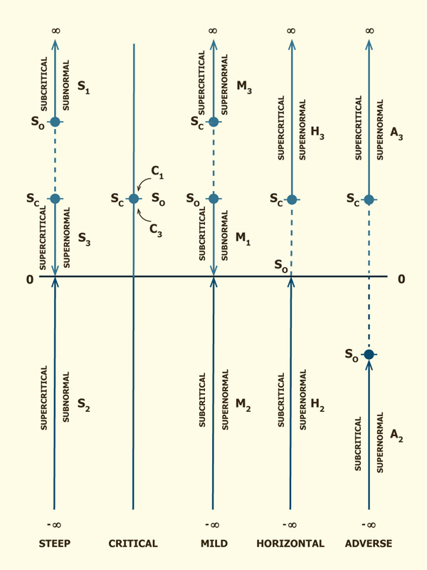Figure 1 shows a graphical representation of flow-depth gradient ranges in the water-surface profiles. The arrow shows the direction of computation. For instance, the depth gradient for the S3 profile (supercritical/supernormal) decreases from Sc (a finite positive value) to 0 (asymptotic to normal flow). Likewise, the depth gradient for the C1 (subcritical/subnormal) and C3 (supercritical/supernormal) profiles is constant and equal to So = Sc . Online water-surface profile calculators are enabled in Table 2. Table 2.  Classification of water-surface profiles. [Click on any profile type on Col. 9 to link to online water-surface profile calculator] No. (1) Sy /Sc (2) Profile (3) So /Sc (4) Slope (5) Depth relations (6) Sy varies Profile type (9) From (7) To (8) 1.  SUBCRITICAL/SUBNORMAL FLOW 1:  1 > F 2 < So / Sc 1 Positive Backwater > 1 Steep y > yc > yn So ∞ S1 2 Positive Backwater = 1 Critical y > yc = yn So = Sc So = Sc C1 3 Positive Backwater < 1; > 0 Mild y > yn = yc So 0 M1 2A.  SUPERCRITICAL/SUBNORMAL FLOW 2:  1 < F 2 < So / Sc 4 Negative Drawdown > 1 Steep yc > y > yn - ∞ 0 S2 2B.  SUBCRITICAL/SUPERNORMAL FLOW 3:  1 > F 2 > So / Sc 5 Negative Drawdown < 1; > 0 Mild yn > y > yc - ∞ 0 M2 6 Negative Drawdown = 0 Horizontal y > yc ; yn → ∞ - ∞ So = 0 H2 7 Negative Drawdown < 0 Adverse y > yc ; yn → ∞ - ∞ So < 0 A2 3.  SUPERCRITICAL/SUPERNORMAL FLOW 4:  1 < F 2 > So / Sc 8 Positive Backwater > 1 Steep yc > yn > y Sc 0 S3 9 Positive Backwater = 1 Critical yc = yn > y So = Sc So = Sc C3 10 Positive Backwater < 1; > 0 Mild yn > yc > y Sc ∞ M3 11 Positive Backwater = 0 Horizontal yc > y ; yn → ∞ Sc ∞ H3 12 Positive Backwater < 0 Adverse yc > y ; yn → ∞ Sc ∞ A3 1 Given that So /Sc > F 2 > 0, no horizontal or adverse profiles are possible in subcritical/subnormal flow. 2 Given that So /Sc > 1, no critical, mild, horizontal or adverse profiles are possible in supercritical/subnormal flow. 3 Given that So /Sc < 1, no steep or critical profiles are possible in subcritical/supernormal flow. 4 Given that So /Sc is not limited, all five profiles are possible in supercritical/supernormal flow. Figure 1.   Graphical representation of flow-depth gradient ranges in water-surface profiles. 4.  SUMMARY The gradually varied flow equation is expressed in terms of the critical slope Sc . In this way, the flow depth gradient dy/dx is shown to be strictly limited to values outside of the range encompassed by So and Sc. This completes the definition of depth-gradient ranges for all water-surface profiles. For instance, the flow-depth gradient for the S3 profile decreases from Sc (a finite positive value) to 0 (asymptotic to normal depth). Likewise, the flow depth gradient for the C1 and C3 profiles is constant and equal to So = Sc. Table 3 shows a summary of water-surface profiles. Online calculators are provided to round up the experience. Table 3.  Summary of water-surface profiles. [Click on any image to enlarge] Family Character Rule So > Sc So = Sc So < Sc So = 0 So < 0 1 Retarded (Backwater) 1 > F 2 < So / Sc S1 C1 M1 - - 2A Accelerated (Drawdown) 1 < F 2 < So / Sc S2 - - - - 2B Accelerated (Drawdown) 1 > F 2 > So / Sc - - M2 H2 A2 3 Retarded (Backwater) 1 < F 2 > So / Sc S3 C3 M3 H3 A3 REFERENCES Chow, V. T. (1959). Open-channel hydraulics. McGraw-Hill, New York. Henderson, F. M. (1966). Open channel flow. MacMillan, New York. USDA Soil Conservation Service. (1971). Classification system for varied flow in prismatic channels. Technical Release No. 47 (TR-47), Washington, D.C.

200417