1. INTRODUCTION This paper reports on a series of tests aimed at developing improved procedures for catchment routing. The objective is to compare kinematic and diffusion models within several scenarios of physical reality and numerical fact. The effects of bed slope and Courant number are specifically isolated herein. 2. BACKGROUND
The kinematic wave equation is the basis of most catchment routing models in current use.
in which Q = flow rate; c = celerity of kinematic waves; qL = lateral inflow, per unit of channel length; x = spatial variable; and t = temporal variable. Equation 1 can be discretized on the x-t plane in several ways. Ponce (3) identified three fully off-centered schemes: (1) Scheme Ι, forward-in-time/backward-in-space, stable for Courant numbers less than 1 and convergent as Courant number increases to 1; (2) Scheme ΙΙ, forward-in-space/backward-in-time, stable for Courant numbers greater than 1 and convergent as Courant number decreases to 1; and (3) Scheme ΙΙΙ, uncoditionally stable but nonconvergent for all Courant numbers. These and other similar schemes have been widely referred to as kinematic wave solutions. Schemes Ι and ΙΙ are complementary; versions of them are in wide use, for instance in the kinematic wave routing option of HEC-1 (1). Scheme ΙΙΙ (and related versions), although nonconvergent, has also been favored because of its feature of unconditional stability (2). Ponce (3) has applied the concept of matched physical and numerical diffusivity to the distributed catchment routing problem. He compared the solution of scheme ΙΙΙ, with its associated "uncontrolled" numerical diffusion, with that of a scheme developed by matching diffusivities (herein referred to as scheme ΙV), under a wide range of grid resolutions. While scheme ΙΙΙ was shown to be highly sensitive to grid size, scheme ΙV was not. This led Ponce to suggest that scheme ΙV was altogether better than scheme ΙΙΙ. In scheme ΙV, the physical diffusivity is given by:
in which ν = physical diffusivity; q = unit-width discharge; and So = bed slope. Matching physical and numerical diffusivities leads to the cell Reynolds number:
in which D = cell Reynolds number; and ∆s = spatial interval (either ∆x or ∆y). By including the Froude number dependence of the physical diffusivity Ponce (3) extended the concept of matched diffusivities to the realm of dynamic waves. This lead to the diffusion-cum-dynamic model (herein referred to as dynamic model), which is the same as scheme ΙV but with cell Reynolds number defined as follows:
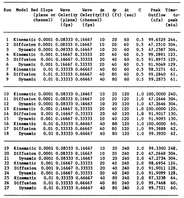
in which β = exponent in the single-valued rating curve (discharge-area relation); and F = Froude number. 3. STUDY STRATEGY The sensitivity of catchment response to routing model, bed slope and Courant number is examined herein. Three routing models are chosen: (1) schemes Ι / ΙΙ, with scheme Ι used for Courant numbers less than or equal to 1 and scheme ΙΙ used for Courant numbers greater than 1, hereafter kinematic wave model; (2) scheme ΙV, with matched physical and numerical diffusivities, hereafter diffusion wave model; and (3) the diffusion-cum-dynamic model, i.e. scheme ΙV, but with Froude-number-dependent diffusivity, hereafter dynamic wave model. In light of Ponce's findings (3), the excessive and uncontrolled numerical diffusion of scheme ΙΙΙ precluded its further consideration. Three bed slopes and three Courant numbers were chosen, encompassing a range of values likely to be encountered in actual practice. The combinations of models, bed slopes and Courant numbers led to a program of twenty-seven (27) runs. 4. NUMERICAL EXPERIMENTS Numerical experiments were designed to test the sensitivity of catchment response to model, bed slope and Courant number. A hypothetical example suited to the overall study objectives was developed. The example consisted of a catchment conceptualized as an open book with two planes adjacent to one channel. The planes are assumed to be impermeable, with rainfall excess (net rainfall) equal to total rainfall. The inflow to the planes is the rainfall excess, and runoff is by overland flow in a direction perpendicular to the channel alignment. Inflow to the channel is by lateral contribution from the planes, and outflow from the channel is the catchment response (3). The dimensions are: plane length (in the direction of plane flow) = 600 ft (183 m); channel length = 1200 ft (366 m). The rainfall is 3 in/hr (76.2 mm/hr), which when multiplied by the catchment area results in a potential maximum peak outflow of 100 cfs (2.83 m3/s). The following values of bed slope were selected: (1) mild, 0.0001; (2) average, 0.001; and (3) steep, 0.01. The chosen Courant numbers were: 0.5, 1 and 2. For these bed slopes and Courant numbers, wave celerities and discrete intervals (∆x, ∆y, and ∆t) were chosen to produce a consistent series of 27 runs (Table 1). Given the catchment geometry, flow path, and wave celerities, rainfall durations were made equal to time-of-concentration, assuming kinematic travel time and neglecting diffusion. Accordingly, for the mild bed slope (0.0001) the rainfall duration was set at 240 minutes, with a runoff volume of 1,440,000 cu ft (40,776 m3); for the average slope (0.001) it was set at 120 minutes, with a runoff volume of 720,000 cu ft (20,388 m3); and for the steep slope (0.01) it was set at 60 minutes, with a runoff volume of 360,000 cu ft (10,914 m3). For this study the β value for plane flow was set at 3, characteristic of laminar flow, while the value for channel flow was set at 1.5, characteristic of turbulent Chezy friction. Mean flow velocities were calculated by dividing wave celerities by β values. Average flow depths were calculated by assuming laminar flow in the planes and turbulent flow in the channels. 5. RESULTS The results of runs 1 through 27, expressed in terms of peak outflow and time-to-peak, are shown in Table 1. These results lead to the following conclusions regarding effect of model, bed slope, and Courant number on catchment response:
6. DIFFUSION EFFECT AND CATCHMENT RESPONSE
The effect of diffusion on catchment response merits further analysis herein. Test results have clearly shown that bed slope (whether of plane or channel) has a significant influence on the amount of physical diffusion experienced by the outflow hydrograph. Further experience with the diffusion model has led to the following conclusions: (1) For steep bed slopes, the hydrograph diffusion is small; for average bed slopes, it is medium; for mild bed slopes, it is large. Other things being equal, the lesser the bed slope, the greater the diffusion effect experienced by the outflow hydrograph; In general, catchment response is a function of the following time parameters: (1) rainfall duration tr; (2) kinematic time-of-concentration tc; and (3) effective time-of-concentration te. For each catchment and rainfall event, there is a potential maximum value of peak outflow, calculated as the product of rainfall intensity and catchment area. Together with rainfall intensity, rainfall duration accounts for the total runoff volume. Kinematic time-of-concentration is similar to the well established concept of time-of-concentration, i.e. the longest time it takes a parcel of water to travel from catchment divide to outlet, neglecting diffusion effects. It accounts for catchment size and shape, mean velocity and boundary friction. Effective time-of-concentration includes the diffusion effect and is generally greater than kinematic time-of-concentration. Depending on the relative values of rainfall duration, kinematic time-of-concentration and effective time-of-concentration, catchment flow can be either kinematic or diffusion flow, and can be either subconcentrated, concentrated, or superconcentrated.
Kinematic Flow is that for which effective time-of-concentration is equal to kinematic Subconcentrated Flow is defined as catchment flow in which rainfall duration is less than effective time-of-concentration; consequently, peak outflow is less than the potential maximum value. Concentrated Flow is defined as catchment flow in which rainfall duration is equal to effective time-of-concentration, with peak outflow equal to the potential maximum value. Superconcentrated Flow is defined as catchment flow in which rainfall duration is greater than effective time-of-concentration; peak outflow is equal to the potential maximum value. 7. DIFFUSION VS DYNAMIC MODELS
It has been shown that diffusion and dynamic models give practically the same results, with little to be gained by using Froude-number-dependent diffusivity in catchment modeling. This behavior,
characteristic of a wide range of bed slopes--from steep to mild--can be explained as follows: 8. SUMMARY AND CONCLUSIONS
Discrete catchment models of kinematic, diffusion and dynamic waves are tested under a wide range of bed slopes and Courant numbers. The kinematic model uses an off-centered discretization of the kinematic wave equation. The diffusion model is formulated by matching physical and numerical diffusivities, which gives it grid independence for a wide range of resolution levels.
Results show the clear advantages of using the diffusion wave technique in lieu of the kinematic wave. The kinematic model fails to account for bed slope effect, rendering it unsuitable as a general model of catchment behavior. The diffusion and dynamic models, however, properly account for bed slope effect, producing hydrograph diffusion as required by the physics of the wave phenomena.
In light of the present findings, the diffusion model is advocated as a general model of catchment behavior. The kinematic model should be used only in cases where the diffusion effect is negligible. Generally, there is very little to gain by using the dynamic model in lieu of the diffusion model. REFERENCES
"HEC-1, Flood Hydrograph Package, Users Manual." 1985. The Hydrologic Engineering Center, U.S. Army Corps of Engineers, Davis, Calif., Sept., 1981, revised Jan., 1985.
Huang, Y. H. 1978. "Channel Routing by Finite Difference Method," Journal of the Hydraulics Division, ASCE, Vol. 104, No. HY10, Oct., 1379-1393.
Ponce, V. M. 1986. "Diffusion Wave Modeling of Catchment Dynamics," Journal of Hydraulic Engineering, ASCE, Vol. 112, No. 8, Aug., 716-727.
|
| 220310 |
| Documents in Portable Document Format (PDF) require Adobe Acrobat Reader 5.0 or higher to view; download Adobe Acrobat Reader. |