Harley et al. (3) effectively incorporated the tracking of shock waves into their catchment model based on the method of characteristics. They treated shock waves as minor disturbances in the regular flow field, and simulated normal characteristics and shock fronts on an equal basis.

More recently, Borah et al. (1) have presented an analytical solution to the kinematic wave approximation for unsteady flow routing. The model allows time-dependent lateral inflow with piecewise spatial uniformity and is designed for use in watershed flow simulation. A significant feature of the Borah et al. model is its explicit capability for routing discontinuities that may develop during the course of the computation. A solution based on the method of characteristics and an approximate shock-fitting scheme preserves the effect of the shocks, and enables the routing of a variety of unsteady flows, ranging from simple cascades to complex natural watersheds.

Other references to the calculation of shocks, kinematic or otherwise, are scattered throughout the literature. For instance, Smith (11) developed a method for predicting the rate of movement and attenuation of kinematic flow over an infiltrating plane. Using a numerical procedure, he was able to document certain shock-type features of flood wave movement under specified initial and boundary conditions. Earlier, Tinney and Bassett (12) had reported on analytical and experimental work to predict the terminal shape of a shallow liquid front. For the turbulent flow case, their findings confirm the importance of the reference channel length, L_o (Eq. 1), in dimensionless studies of unsteady open-channel flow phenomena.

Although the concept of kinematic shock is well established in the field of watershed modeling, its transposition to streamflow routing remains a subject of controversy. A few investigators, most notably Cunge (2), have gone as far as to question its existence altogether. There is no doubt that the steepening tendency is real. Whether the unsteady gradually varied flow equations can continue to describe the phenomena in the vicinity of the shock remains to be determined. On more practical grounds, it would be of interest to determine the flow and channel characteristics that will tend either to promote or to inhibit the development of kinematic shock. Such a line of inquiry is pursued in this paper.

3.  METHODOLOGY

The approach used herein to study the potential for kinematic shock development consists of the following: (1) Identification of the relevant flow and channel parameters; (2) selection of parameter ranges; (3) selection of a physically based flow routing model; and (4) development of a strategy for testing the sensitivity of the chosen parameters to kinematic shock development under a wide range of conditions.

Parameter Identification. In unsteady open channel flow theory, two parameters characterize linear wave movement in wide channels (6): (1) the reference flow Froude number, F_o = u_o / (g d_o)^1/2 ; and (2) the dimensionless wave number σ = 2π (L_o / L), in which u_o, and d_o = reference flow mean velocity and depth, respectively; g = gravitational acceleration; and L = wavelength. The Froude number contains information on the channel bed slope and frictional characteristics, while the dimensionless wave number relates the length scales of wave, L and reference flow, L_o. Additional parameters are needed in real-world applications to account for relative wave height and allow for the specification of any arbitrary cross-sectional shape. To account for wave height (as well as overall hydrograph shape), it is necessary to select a type of inflow hydrograph. In this study a gamma function is chosen as the standard inflow hydrograph shape. The equation for the gamma function is of the following form (9):

t                tp - t      Qt  = Qb + (Qp - Qb) ( ____) exp( ______ )                                      tp              tg - tp

(2)

in which Q_t = inflow at time t; Q_b = baseflow; Q_p = peak inflow; t_p = time-to-peak of inflow hydrograph; t_g = time-to-center-of-gravity of inflow hydrograph; and r = t_p / (t_g - t_p).

Given the aforementioned, the ratio of base-to-peak inflow, Q_b / Q_p, was chosen as an indicator of relative wave height, and the time-to-peak t_p was chosen to depict overall hydrograph time scale.

With regards to the cross-sectional shape parameters, the ones chosen here are those normally used in kinematic wave routing applications: the coefficient α and exponent β in the power fit to the single-valued discharge-flow area relation:

Q = α A β

(3)

in which Q = discharge; and A = flow area, based on a suitable uniform flow formula (such as Manning's or Chézy's).

Parameter Ranges. The testing program was designed to vary the chosen parameters within suitable ranges. To account for the Froude number variation, a matrix of five bed slopes, S_o , and five values of Manning's n was established, leading to a framework of 25 channels, each with a unique set of S_o and n. Adopted values of S_o , were: 0.01, 0.004, 0.001, 0.0004, and 0.0001; values of n were: 0.01, 0.02, 0.04, 0.08, and 0.10. Mild bed slopes with large Manning's n led to low Froude number flows, while steep bed slopes with small Manning's n resulted in high (even larger than unity) Froude number flows.

In nonlinear flood waves, the steepening of the rising limb tends to be counteracted by the diffusive effects brought upon by the dynamic components. As shown by Ponce and Simons (6), the dimensionless wave number, σ, is an indicator of the relative size of the dynamic components. Accordingly, in order to guarantee a sufficient amount of wave steepening, unimpaired by the dynamic effect, the tested waves were chosen to remain within the realm of kinematic and diffusion waves (generally, low σ values). For this purpose, the time-to-peak, t_p of the inflow hydrograph, an indicator of overall time wale, was used to test the satisfaction of the diffusion wave criterion developed by Ponce et al. (7) and subsequently modified (10) for application to gamma hydrographs:

g N = tp So (___ )1/2  ≥ 15                   do

(4)

in which N = dimensionless number; g = gravitational acceleration; and all other variables are as previously defined. For each specified flow condition, the satisfaction of Eq. 4 guarantees that the tested wave is properly a kinematic/diffusion wave, and therefore, largely free of very strong diffusive effects that would tend to counteract the development of kinematic shock.

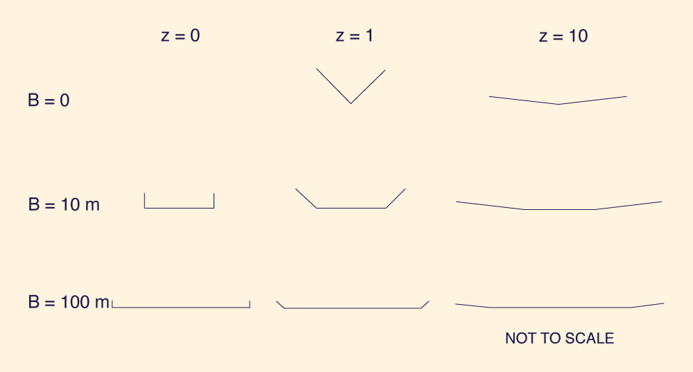
Fig. 1. Rectangular/trapezoidal/triangular cross sections used in this study

The effect of relative wave height was accounted for by varying the ratio of base-to-peak flow. Two ratios were chosen for this study: (1) A low value, Q_b /Q_p = 0.05 (labeled L); and (2) a high value, Q_b /Q_p = 0.50 (labeled H).

A complete accounting of the variation of cross-sectional shape parameters, α and β, was deemed too ambitious. A limited yet meaningful program was devised by selecting a family of rectangular/trapezoidal/ hiangular cross sections, using three bottom widths and three side slopes (Fig. I). The bottom widths chosen were B = 0, 10, and 100 m; the side slopes were z = 0, 1, and 10 (0 = horizontal: 1 = vertical). This led to eight channels (the case of B = 0 and z = 0 being trivial) encompassing a wide range of cross-sectional shape parameters. In general, the β value is allowed to vary from the theoretical (Manning friction) β = 1.667 for wide channels of rectangular cross-sectional shape (B = 100 and z = 0), to β = 1.333 for triangular-shaped channels (B = 0 and z = 1). The exception is the case of narrow, rectangular channels (B = 10, z = 0) coupled with low Froude numbers flows (large flow depths) for which the β value approaches 1. The above eight channels were considered to provide a sufficiently wide range of β to allow meaningful conclusions to be drawn from the sensitivity analysis.

Model Selection. The SYS75 model was selected as the numerical model to carry out the present study. This model is a computer program developed by the senior writer featuring a physically based coeffident routing module in which the routing parameters are allowed to vary in time and space (8). This gives it the capability for routing nonlinear flood waves, and therefore, the ability to study the wave steepening caused by the nonlinearity. The computer model can calculate discharge, flow area, and stage discretely in space and time, when presented with ap-propriate initial and boundary conditions. The accuracy of the SYS75 model has been extensively documented (10), and it is considered to be adequate for the routing of kinematic and diffusion waves. Additional details on the SYS75 model are given elsewhere (10).

Study Strategy. The overall strategy for accomplishing the study objectives consists of the following: (1) establishing a standardized channel length based on total inflow volume and peak flow area above base flow, to enable shocks to be analyzed at comparable stages of development; (2) routing the hydrographs from the upstream to the downstream end of the channel by using the SY575 model; and (3) comparing the slope of the-rising limb of the outflow hydrograph, S_ro, with that of the rising limb of the inflow hydrograph, S_ri, (the slope is taken as a change in discharge per unit of time, approximately at midpoint of the rising limb). The ratio S_ro /S_ri is interpreted as a measure of the potential for shock development.

In addition, other manifestations of the shock presence such as numerical instabilities are documented as part of the study.

4.  TESTING PROGRAM

Seven channels, each with a unique set of bed slope, S_o and Manning's n, were selected as part of this study. For identification purposes, they were given alphabetic names from A-G, followed by an L or H, depicting either low or high base-to-peak inflow ratio. Channel F was tested under both L and H conditions, and channel G was tested under three different t_p ratios, for a total of ten series (Table 1). Each series was tested with eight cross-sectional shapes (Fig. 1), making a total of eighty (80) computer runs.

Table 1.  Test series. Bed slope, So (1) Manning's friction coefficient, n ( Fpi , Peak inflow Froude number) 0.01 (2) 0.02 (3) 0.04 (4) 0.08 (5) 0.10 (6) 0.01 DH (2.45) AL (0.26) 0.004 FL, FH (0.70, 0.87) 0.001 BH (0.26) 0.0004 GL, GL1, GL2 (0.10) 0.0001 CL (0.34) EH (0.04)

For each series, the total channel length is standardized with respect to the inflow volume. The inflow hydrograph volume above baseflow V_I , is calculated by the following formula (10):

m! VI = ______ em (Qp - Qb )tp          mm+1

(5)

in which m = t_p (t_g - t_p) is an integer. The channel length, L_c is estimated by the following formula (10):

VI Lc = ______           Apr

(6)

in which A_pr = flow area corresponding to Q_pr = Q_s - Q_b. Equation 6 guarantees that the routing length L_c is related to the inflow hydrograph volume, and therefore, remains physically meaningful for kinematic shock comparative studies. Inflow hydrograph and channel characteristics for the ten series tested herein are given in Table 2.

Table 2.  Inflow hydrograph and channel characteristics. Channel (1) Qb , base flow, in cubic meters per second (2) Qp , base flow, in cubic meters per second (3) tp , time-to-peak of inflow hydrograph, in seconds (4) tg , time-to-center of gravity of inflow hydrographs, in seconds (5) VI , inflow hydrograph volume above base flow, in cubic meters (6) Lc , channel length in meters (7) AL 1.25 25 900 1,200 31,802 1,000 BH 100 200 14,400 21,600 2,660,060 45,000 CL 25 500 172,800 345,600 223,116,572 1,000,000 DH 50 100 3,600 5,400 332,508 45,000 EH 250 500 172,800 259,200 79,801,806 200,000 FL 2.5 50 3,600 5,400 315,882 12,000 FH 50 100 3,600 5,400 332,508 20,000 GL 125 2,500 57,600 86,400 252,705,719 160,000 GL1 125 2,500 115,200 172,800 505,411,438 320,000 GL2 125 2,500 230,400 345,600 1,010,822,876 640,000

5.  RESULTS

Results for all eighty (80) runs are summarized in Tables 3 and 4. For the sake of clarity, all runs are hereafter referred to by their row and column identification shown in these tables. For instance, run 34 would correspond to row 3 (channel with B = 10 and z = 0) and column 4 (EH series).

Table 3.  Rating curve parameters α and β. Para- meter (1) Row (2) B (3) z (4) Column 0 1 2 3 4 5 6 7 Channel AL (5) BH (6) CL (7) DH (8) EH (9) FL (10) FH (11) GLa (12) α 1 0 1 0.500 0.395 0.500 5.000 0.050 1.581 1.581 0.125 2 0 10 0.291 0.230 0.291 2.913 0.029 0.921 0.921 0.073 3 10 0 0.239 0.564 0.603 2.933 0.236 0.722 0.935 0.529 4 10 1 0.239 0.342 0.398 2.419 0.053 0.725 0.910 0.132 5 10 10 0.231 0.222 0.276 2.365 0.029 0.702 0.815 0.072 6 100 0 0.047 0.039 0.049 0.467 0.008 0.147 0.149 0.020 7 100 1 0.047 0.041 0.051 0.467 0.009 0.147 0.150 0.021 8 100 10 0.049 0.060 0.071 0.488 0.018 0.152 0.167 0.041 β 1 0 1 1.333 1.333 1.333 1.333 1.333 1.333 1.333 1.333 2 0 10 1.333 1.333 1.333 1.333 1.333 1.333 1.333 1.333 3 10 0 1.563 1.247 1.278 1.567 1.025 1.586 1.486 1.040 4 10 1 1.548 1.369 1.385 1.549 1.326 1.570 1.482 1.328 5 10 10 1.397 1.339 1.342 1.392 1.333 1.415 1.361 1.334 6 100 0 1.664 1.648 1.649 1.664 1.562 1.664 1.661 1.571 7 100 1 1.663 1.640 1.643 1.663 1.544 1.663 1.658 1.555 8 100 10 1.640 1.537 1.548 1.641 1.390 1.646 1.618 1.403 a All GL channels (GL, GL1, y GL2) have the same value of α and β Note: B = bottom width (m); z = side slope (z H: 1 V)

Table 4.  Final-slope-to-initial slope ratios Sro / Sri. Row (1) B (2) z (3) Column 0 1 2 3 4 5 6 7 8 9 Channel AL (4) BH (5) CL (6) DH (7) EH (8) FL (9) FH (10) GL (11) GL1 (12) GL2 (13) 1 0 1 1.02 0.61 1.18 1.32 0.31 2.73 1.27 0.42 0.73 1.17 2 0 10 1.24 0.72 1.80 1.45 0.25 3.95 1.40 0.52 1.08 1.98 3 10 0 2.15 0.46 0.59 1.45 0.88 4.00 1.40 0.26 0.04 0.05 4 10 1 2.15 0.69 1.71 1.61 0.31 3.75 1.40 0.45 0.77 1.22 5 10 10 1.47 0.76 2.32 1.71 0.25 4.00 1.47 0.52 1.09 1.77 6 100 0 3.96 0.90 2.95 2.24 0.34 4.90 2.00 0.81 1.70 2.92 7 100 1 3.73 0.91 2.76 2.42 0.35 5.00 2.00 0.94 1.85 2.79 8 100 10 3.20 0.91 2.97 2.64 0.26 6.00 2.33 0.67 1.35 2.79 Note: B = bottom width (m); z = side slope (z H : 1 V)

Table 3 shows rating curve parameters α and β for all runs. The value of α accounts largely for channel bed slope and bottom friction, and to a lesser extent for the effect of wetted perimeter on cross-sectional shape. The value of β accounts for cross-sectional shape and the type of bottom friction (whether Manning or Chézy). Values of α vary from α = 0.008 (run 64) to α = 5.000 (run 13); values of β varies from β = 1.025 (run 34) to β = 1.664 (run 60). Table 3 shows that β varies generally from the theoretical β = 1.333 for triangular channels (β = 0) with Manning friction, to values close to the theoretical (β = 1.667 for wide rectangular channels (β = 100 and z = 0) with Manning friction. Values of β outside the above range are calculated for narrow channels with relatively large flow depths (low Froude number flows); see for instance, values of β for runs 34 and 37.

Table 4 shows final slope to initial slope ratios S_ro / S_ri for all 80 runs. These are ratios of slopes of the rising limb of outflow and inflow hydrographs, respectively. Therefore, the higher the ratio, the more marked the tendency for shock development within the standardized channel length. These results lead to the following conclusions:

1. All parameters have a definite effect on shock development. The slope ratio, S_ro / S_ri, is directly proportional to the peak inflow Froude number (channel friction and bed slope), time-to-peak t_p, (overall wave time scale), and β value (cross-sectional shape, and to a lesser extent, type of channel friction); and inversely proportional to the ratio Q_b / Q_p (relative wave height).

2. The time scale (and therefore, length scale) of the wave is directly related to wave steepening, as shown by the results of channels GL, GL1, and GL2. As t_p increases from GL to GL1 and GL2, the wave becomes more kinematic and therefore, more prone to shock development (see for instance, column 9 as compared to column 8). The exception to this pattern is given by runs 37-39, confirming the odd behavior of this particularly narrow channel with a β value near 1. Values of the slope ratio less than 1 (see column 7) indicate wave diffusion instead of wave steepening, signaling the complete absence of the shock.

3. The Froude number has a definite effect on wave steepening, as shown by comparing results of columns 5 (channel FL, Froude number = 0.7) and 9 (channel CL2, Froude number = 0.1) having the same Q_b /Q_p, ratio (Q_b = 0.05) and approximately the same N value (see Eq. 4). For instance, run 85 shows a slope ratio of 6.0, as compared with 2.79 for run 89.

4. Cross-sectional shape as embodied in the β value has also a definite influence on wave steepening. Wide channels (rows 6-8) having β values approaching 1.667 show a much stronger tendency for wave steepening than either triangular (rows 1 and 2, β = 1.333) or narrow (rows 3-5, β generally between 1.333 and 1.667). The exception, runs 37-39, show very strong wave diffusion due to their low β value (β = 1.04).

5. The ratio of base-to-peak inflow, Q_b / Q_p has a definite effect on wave steepening, m shown by the results of columns 5 and 6, Table 4. The L flow condition consistency produced a larger slope ratio than the H flow condition (see for instance run 75, having a slope ratio of 5.0, as compared to run 76, with a slope ratio of 2.0).

Fig. 2   Typical outflow hydrograph: (a) run 45, showing marked steepening and associated numerical instabillity; (b) run 69, showing mild wave steeping; (c) run 47, showing wave diffusion instead of wave steeping.

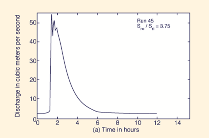
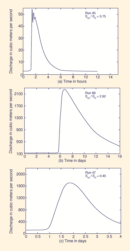
Figure 2 shows typical outflow hydrographs: run 45, showing marked steepening and associated numerical instability [Fig. 2(a)]; run 69, an intermediate case showing some wave steepening [Fig. 2(b)] and run 47, the other extreme, shelving wave diffusion instead of wave steepening [Fig. 2(c)].

---

6.  SUMMARY AND CONCLUSIONS

A series of numerical experiments has been performed to determine the flow and channel characteristics that are most conducive to kinematic wave steepening and associated kinematic shock phenomena. Relevant flow and channel characteristics are identified at the outset, and a program of 80 computer runs is completed, varying the inflow hydrograph peak Froude number, time-to-peak, base-to-peak flow ratio, and the channel cross-sectional shape. Standardized channel lengths are calculated to enable the analysis of shocks at comparable stages of development. Gamma hydrograph inflows are routed from upstream to downstream using a physically based flow routing computer model.

It is found that the inflow hydrograph peak Froude number, F_pi , time-to-peak, t_p and base-to-peak flow ratio, Q_b / Q_p and the cross-sectional shape parameter, β, all have a definite effect on kinematic shock development. The size of the wave is perhaps mostly responsible for the occurrence or nonoccurrence of the shock. Kinematic waves (as opposed to diffusion waves) are more prone to shock development, as are waves with a low Q_b / Q_p ratio. High Froude number flows are somewhat more conducive to shock development than low Froude number flows. Wide rectangular channels show a much stronger tendency for wave steepening than either triangular or narrow channels. Low values of β (β approaching 1.0) increase wave diffusion and inhibit shock development.

Given the foregoing results, it is concluded that kinematic shock will be most likely to occur under the following conditions: (1) A kinematic wave; (2) a low base-to-peak flow ratio; (3) a high Froude number flow; and (4) a wide and sufficiently long channel. Whether all these conditions are met remains to be assessed for individual cases. For example, a flood wave traveling in a steep, initially dry channel satisfies most of these conditions, making it a likely case for shock development. As another example, when using a kinematic wave routing method, the first condition above is automatically met by the method's assumption. Therefore, in this case it is only necessary to satisfy the other three remaining conditions for shock development.

The preceding findings can help to explain the demonstrated absence of kinematic shock in flood plain routing computations. As water levels lise above flood stage, the wetted perimeter increases at a faster rate than for inbank flows, triggering a decrease in the value of β. This effectively counteracts the steepening tendency and arrests kinematic shock development.

---

APPENDIX I.  REFERENCES

1. Borah, D. K., N. Prasad, N., and C. Alonso. 1980. "Kinematic wave routing incorporating shock fitting," Water Resources Research, Vol. 16, No. 3, June, 529-541.

2. Cunge, J. A. 1969. "On the subject of a flood propagation computation method (Muskingum method)," Journal of Hydraulic Research, Vol. 7, No. 2, 205-230.

3. Harley, B. M., F. E. Perkins, and P. S. Eagleson. 1970. "A modular distributed model of catchment dynamics," Report No. 133, Ralph M. Parsons Laboratory for Water Resources and Hydrodynamics, Massachusetts Institute of Technology, Cambridge, Mass., Dec.

4. Kibler, D.F, and D. A. Woolhiser. "The kinematic cascade as a hydrologic model," Hydrology Paper No. 39, Colorado State University, Fort Collins, Colo.,

5. Lighthill, M. J., and G. B. Whitham. 1955. "On kinematic waves. I. Flood movement in long rivers," Proceedings, Royal Society of London, Vol. 4229, May, 281-316.

6. Ponce, V. M., and D. B. Simons. 1977. "Shallow wave propagation in open channel flow," Journal of the Hydraulics Division, ASCE, Vol. 103, No. HY12, Dec., 1461-1976.

7. Ponce, V. M., R. M. Li, and D. B. Simons. 1978. "Applicability of kinematic and diffusion models," Journal of the Hydraulics Division, ASCE, Vol. 104, No. HY3, Mar., 353-360.

8. Ponce, V. M., and V. Yevyevich, V. 1978. "Muskingum-Cunge method with variable parameters," Journal of the Hydraulic Division, ASCE, Vol. 104, No. HY12, Dec., 1663-1667.

9. Ponce, V. M., and F. D. Theurer, F. D. 1982. "Accuracy criteria in diffusion routing," Journal of the Hydraulics Division, ASCE, Vol. 108, No. HY6, June, 747-757.

10. Ponce, V. M., 1981. "Accuracy of physically based coefficient methods of flood routing," San Diego State University Civil Engineering Series, No. 83150, Aug.

11. Smith, R. E. "Border irrigation advance and ephemeral flood waves," Journal of the irrigation and Drainage Division, ASCE, Vol. 98, No. IR2, June, 289-307.

12. Tinney, E.R., and D. L. Bassett. 1951. "Terminal shape of a shallow liquid Front," Journal of the Hydraulics Division, ASCE, Vol. 87, No. HY5, Sept., 117-133.

---

APPENDIX II.  NOTATION

The following symbols are used in this payer:

A = flow area;

A_pr = flow area corresponding to Q_pr;

B = bottom width;

d_o = reference flow depth;

F = Fronde number;

F_o = reference flow Froude number;

F = peak inflow Froude number;

g = gravitational acceleration;

L = wavelength;

L_c, = channel length, estimated by Eq. 6;

L_o, = reference channel length, Eq. 1;

m = integer t_p / (t_g - t_p);

N = dimensionless number, Eq. 9;

n = Manning's friction coefficient;

P_s = shock parameter;

Q = discharge;

Q_b = baseflow;

Q_p = peak inflow;

Q_pr = Q_p - Q_b;

Q_t = inflow at time t;

r = ratio t_p /(t_g - t_p );

S_o = channel bed slope;

S_ri = slope of rising limb of inflow hydrograph, L³ / T ² units;

S_ro = slope of rising limb of outflow hydrograph, L³ / T ² units;

t = time;

t_g = time-to-center-of-gravity of inflow hydrograph;

t_p = time-to-peak of inflow hydrograph;

μ_o = reference flow mean velocity;

V_I = inflow hydrograph volume above base flow, Eq. 5;

z = channel side slope (z horizontal - 1 vertical);

α = coefficient in Q-A relation, Eq. 3;

β = exponent in Q-A relation, Eq. 3; and

σ = dimensionless wave number, σ = 2π (L_o / L).

---