|
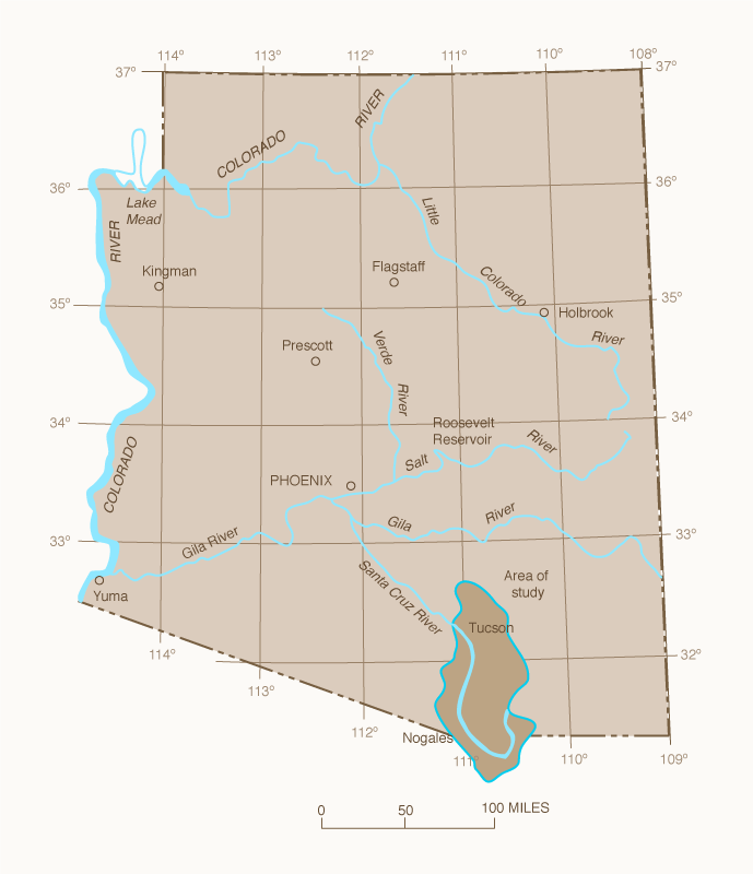
This case study encompasses the upper Santa Cruz River basin, defined as that part of the Santa Cruz basin upstream of Cortaro Farms Bridge, Arizona, and occupying 3,503 square miles (9,073 km2) in southeastern Arizona and northern Sonora, Mexico (Figs. 1 and 2).
The basin is characterized by isolated mountain blocks separated by broad alluvial valleys.
The altitude of the valleys ranges from 2,100-4,700 ft (640-1,432 m) above mean sea level, and the mountains rise to 9,400 ft (2,865 m) above mean sea level (8).
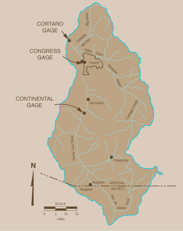
The Santa Cruz river heads in the Huachuca and Patagonia mountains in southeastern Arizona, and flows south past Lochiel into Sonora, Mexico.
In Mexico it changes course, flowing northwestward, reentering Arizona east of Nogales and continuing north towards Tucson.
At Tucson, the river is joined by a major tributary, Rillito Creek; downstream of Tucson, it is joined by the Cañada del Oro, another major tributary heading in the Santa Catalina Mountains, which limit the basin to the northeast.
|
Fig. 1 Geographical location of this study.
|
|
Fig. 2 Santa Cruz
basin and stream configuration.
|
Precipitation varies greatly from year to year, with an average annual rainfall of 14 in. (355.6 mm).
Summer precipitation is usually of high intensity and short duration, resulting from thunderstorms covering small areas.
Winter precipitation is mainly the result of frontal activity, usually covering most of the basin with less intense but longer-lasting storms.
Both summer and winter events are responsible for flooding along the various streams and washes of the Santa Cruz basin.
Most streams in the upper Santa Cruz basin are ephemeral, being dry for long periods of time.
Flow in the streams occurs in direct response to precipitation, except in isolated cases.
The streambeds are extremely permeable, and large amounts of water are lost to the subsurface as the flow moves downstream.
Part of the water lost to infiltration reaches the water table, and water levels in wells near the river also fluctuate in direct response to precipitation (8).
The arid and semiarid conditions characteristic of the basin are highly conducive to quick runoff response, the sparse vegetation doing little to impede runoff.
However, flood peaks are reduced by the relatively large capacity for streambed infiltration.
3. THE EVENT
During the last week of September 1983, a trough at 500 mb remained offshore of California.
This system was combined with a tropical storm, which came very close to Baja California, Mexico.
The combination of the very high moisture fluxes from the tropical storm, towards the region of low pressure off the coast of California, led to a steady, long-lasting, widespread rainfall event over southeastern Arizona (1, 6).
Raingage records indicate that an average of 6 to 8 in. (152.4 to 203.2 mm) of rain fell over large portions of Santa Cruz and neighboring basins in the 6-day period from September 28 to October 3, 1983.
This event contributed to the new all-time yearly total for southeastern Arizona of 25.01 in. (635.2 mm).
The intense rainfalls triggered new record flows on the San Francisco river at Clifton [90,900 cfs (2,572 m3/s)], the Gila river at Safford [132,000 cfs (3,756 m3/s)], and the Santa Cruz river at Tucson [52,700 cfs (1,491 m3/s)].
Flood damage caused by the flooding of the Santa Cruz river and related tributaries included severe bank erosion, which led to structural damage to numerous bridges and their approaches; the collapse of several homes, which fell into the streams; failure of many forms of bank protection; and overbank flooding, which inundated homes with water and sediment.
Overall flood damage estimates range in the neighborhood of $500,000,000 (6).
4. THE PROJECT
In light of the record floods of October 1983, a fresh appraisal of the surface water hydrology of the Santa Cruz basin was indicated.
The evaluation seeks to determine 100-yr frequency floods at the following USGS gaging stations: Continental, Tucson (Congress Street) and Cortaro Farms Bridge. Continental and Cortaro Farms are the sites of bridge improvement projects currently being designed by Pima County.
The Continental, Congress and Cortaro gages have 37, 80 and 44 years of record, and drain 1,682 square miles (4,356 km2), 2,222 square miles (5,755 km2) and 3,503 square miles (9,073 km2), respectively; the Cortaro gage being the downstream point in this case study.
Prior to the flood of October 1983, the maximum USGS flows of record were 26,500 cfs (750 m3/s), 23,700 cfs (671 m3/s), and 23,000 cfs (651 m3/s),
respectively (46, 48, 49).
Peak flows during the flood of October 1983 were estimated by USGS to be 45,000 cfs (1,273 m3/s) at the Continental gage, 52,700 cfs (1,491 m3/s) at the Congress gage, and 65,000 cfs (1,840 m3/s) at Cortaro.
Note that because of the washout of the gage during the October 1983 flood, the Cortaro estimate is subject to a degree of uncertainty.
5. MODELING STRATEGY
General
The strategy for this case study consists of using a deterministic hydrologic simulation model to calculate peak flows at the three locations of interest (Continental, Congress and Cortaro) using rainfall events of 100-yr frequency.
Given the basin's size (3,503 square miles) the choice of spatial and temporal distribution of the input storm is considered to be the most critical modeling decision.
Regional rainfall patterns (3, 24-27, 29, 35) indicate that, for a basin of this size, it is necessary to consider a combination of general and local storms. General (winter) storms are usually of low intensity but tend to cover most of the basin.
Local (summer) storms are concentrated in smaller areas but are commonly of high intensity.
Accordingly, a general storm (in the context of this study) is defined as one covering the whole basin with a rainfall depth distributed uniformly in time.
A local storm is defined as one covering selected portions of the basin
[approximately 400 square miles (1,036 km2)] critically positioned to produce peak flows in strategic locations.
The Soil Conservation Service (SCS) standard dimensionless temporal storm distribution (23) is used to develop a hyetograph for local storms.
Other commonly used distributions, such as SCS Types II and IIA (7, 51) were rejected because of their intended use with storms covering much smaller areas than those considered for this study.
In determining rainfall durations, the time of concentration for the entire basin for a 100-yr frequency flood event was taken into account.
This was estimated at approximately 24 hr. Accordingly, durations of 24, 48 and 96 hr were chosen for the storm simulations.
National Weather Service (NWS) point rainfall depths of 100-yr frequency and the indicated durations were obtained from the appropriate references (34, 47).
Depth-Area Relations
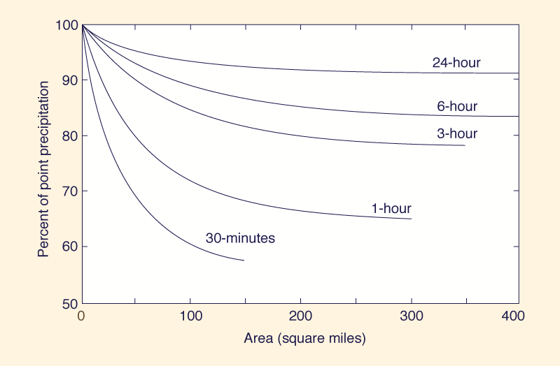
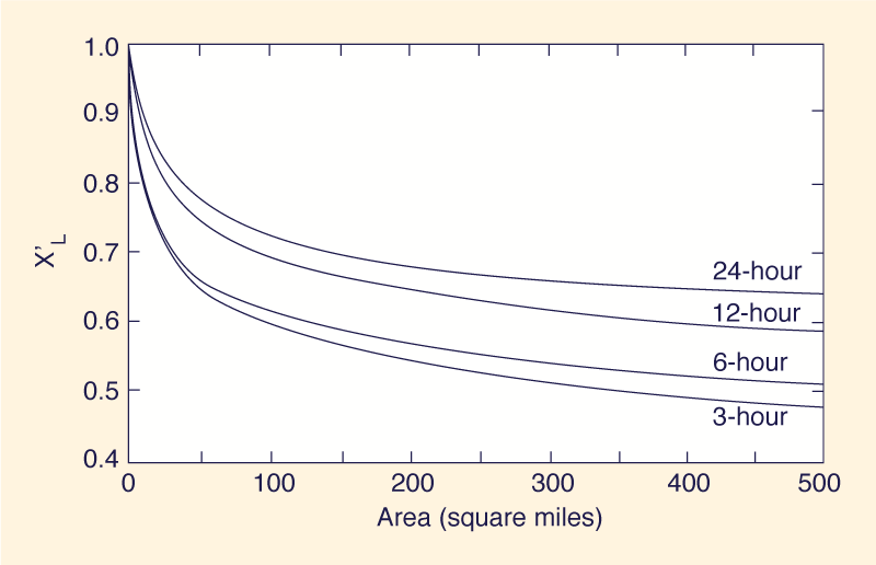
An important consideration in this case study is the choice of depth-area relations.
These are empirical curves which decrease point rainfall depths to account for the extent of areal storm coverage.
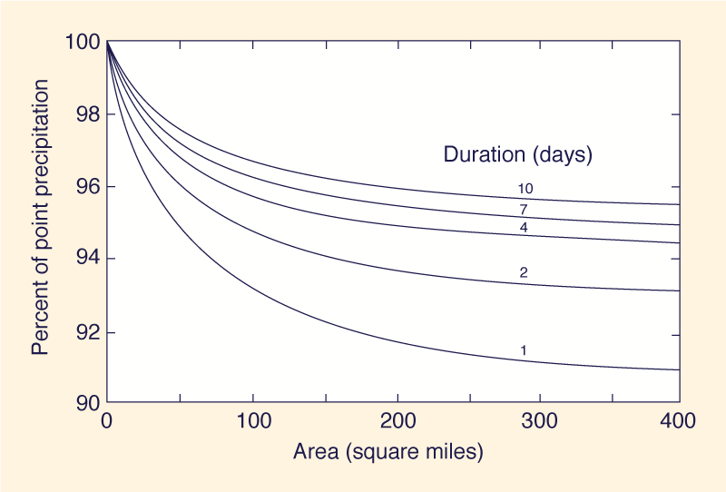
Generalized NWS depth-area relations for the contiguous United States (Figs. 3 and 4) are strictly applicable to basins less than 400 square miles (1,035 km2) (34, 47).
For 400 square miles (local storms in the context of this study), values of 0.91, 0.932 and 0.943 for 24-, 48- and 96-hr storms, respectively, are obtained from these figures.
Since these depth-area relations are asymptotic at 400 square miles,
the extrapolation to 3,503 square miles (for general storms) would leave these values essentially unchanged.
|
Fig. 3 30-minute to 24-hr
NWS depth-area relation (34).
|
|
Fig. 4 2 to 10-day NWS depth-area relation (47).
|
The foregoing areal correction factors are regarded as somewhat conservative for large basins.
Evidence to substantiate this assertion can be found in Ref. 35, which contains regional depth-area relations up to 5,000 sq mi., to be used with estimations of convergence and orographic PMP.
These, however, were derived by analyzing data from PMP-type storms and are therefore strictly applicable to PMP determinations.
Further evidence of the conservatism of the generalized NWS depth-area relations, at least for the semiarid southwest, can be found in a recent NOAA report (9).
This study presents new depth-area relations for frequency-based floods, for 3- to 24-hr storms, for areas up to 500 square miles, applicable to the semiarid southwest (Fig. 5).
Whether these depth-area relations can be extrapolated to larger basins and longer storm durations remains to be ascertained.
|
Fig. 5 2.54-Year
depth-area relation for Southeast Arizona (9).
|
Model Calibration
The model was calibrated by attempting to reproduce the October 1983 flood in a procedure referred to as hindcasting.
Baseline values of runoff curve numbers and streambed infiltration rates were carefully adjusted in order to match calculated and recorded flows.
The adjusted values of these parameters were subsequently used in the general and local storm simulations.
6. MODEL OVERVIEW
The model used in this study is a comprehensive computer-based modeling system to simulate rainfall-runoff processes in complex watersheds and river basins.
The model user specifies the entire stream network at the start, regardless of its complexity, in terms of a set of topological numbers.
Based on these numbers, the calculations proceed in time and space, making the subwatershed hydrograph generation and the routing of flows through stream channels and reservoirs possible.
The total basin area is subdivided into: (1) upland subwatersheds, neighboring the basin perimeter and generating inflow hydrographs to the stream network; and (2) reach subwatersheds, adjacent to stream channel reaches and generating lateral inflow to them.
Subwatershed Hydrograph Generation
Established SCS methodologies are used for subwatershed hydrograph generation (23).
For subwatershed areas less than 6.2 square miles, the watershed time lag is estimated by the curve number method (22).
Otherwise, the time lag is estimated as 60% of the time of concentration.
Following SCS criteria, the unit hydrograph duration is calculated as 2/9 of the time lag.
The unit hydrograph "time to peak" is calculated as five times the unit hydrograph duration.
Using the SCS dimension-less unit hydrograph formula, the peak flow is calculated based on the subwatershed area and the unit hydrograph time-to-peak.
The calculated unit hydrograph is convoluted with the effective storm pattern to generate the outflow hydrograph at each subwatershed outlet.
Stream Channel Routing
The stream channel routing method is a version of the Muskingum-Cunge method (30-33), which has the inherent advantage of being physically based.
In actual practice, this means that the cumbersome and time-consuming subreach parameter calibration
[necessary in conventional hydrologic models such as HEC-1 (15) or TR-20 (7)] is all but eliminated, albeit at the expense of increased physical data requirements.
This enables the modeling of complex stream networks at a level of simulation detail hitherto possible only at a prohibitive cost.
Unlike the classic Muskingum, the calculation of the routing parameters in the Muskingum-Cunge method is based on local flow values, channel cross sections and stream gradients.
This enables the flood wave speed and diffusivity to be expressed in terms of the channel and flow variables, while circumventing the need to handle large amounts of rainfall-runoff data to ascertain the values of these parameters.
In this way, numerous yet accurate routings are possible.
A unique feature of the channel routing module is its capability to route flows with parameters that vary in time as a function of the local flow values (31).
This feature is useful for routing overbank flows, since the routing parameters are recalculated at every time step to adjust more closely to the cross-sectional shape and rating curve.
Channel transmission losses are accounted for in the subreach routing process (32).
This feature is particularly important for this case study, where streambed infiltration constitutes an important component of the overall hydrology of the basin.
Reservoir Routing
The reservoir routing module is based on the storage-indication technique.
The model accepts sets of elevation-storage-outflow values for each reservoir or channel impoundment and uses this information, together with an initial condition, to calculate the outflow hydrograph for the reservoir.
7. DATA REQUIREMENTS
With conventional models, such as HEC-1 or TR-20, historical flow measurements in a few selected reaches are used to "calibrate" reach routing parameters.
In turn, these parameters are "transposed" to other reaches for which historic data is not available.
This procedure assumes, quite practically but nevertheless erroneously, that the flood wave travel and diffusivity characteristics for one reach are transposable to one or more neighboring reaches.
The aforementioned difficulties are altogether eliminated in the model described herein.
Admittedly, the model is highly data-intensive, but with the definite advantage that the data is physical rather than historical in nature.
This considerably reduces the number of "knobs" that the hydrologist has at his/her disposal, leading to more consistent and better modeling practice.
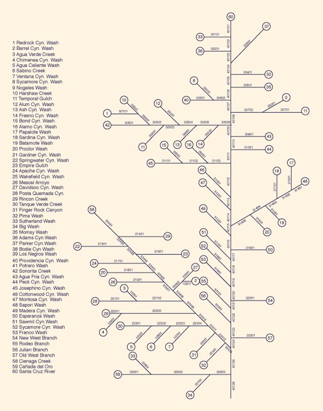
The entire project area and associated stream network was configured into 119 reaches and 179 subwatershed units:
60 upland and 119 reach subwatersheds (Fig. 6).
Each reach was given a five-digit topological number and each upland subwatershed a sequential number.
Within each reach, spatial variability was accounted for by further subdivision into a number of subreaches (usually two or three), each with its own cross-sectional data.
|
Fig. 6 Santa Cruz basin topology.
|
Geometric Data
Subwatershed areas, stream delineation, hydraulic lengths and stream slopes were evaluated using USGS 7.5- and 15-min quadrangle maps.
Cross-sectional coordinate data for 189 cross sections were compiled from different sources (10-13), including actual measurements in remote locations.
Soil and Vegetation Data
Soil and vegetation data were assembled from publications of the USDA SCS (94, 45) and the U.S. International Boundary and Water Commission.
These data were evaluated for vegetative cover types, land use and hydrologic condition, and used to determine subwatershed parameters indicative of runoff potential.
Hydrologic Data
Runoff parameters were obtained from various sources, including local, state and federal agencies (43, 51).
Soil and vegetation maps were used to determine hydrologic soil-cover complexes following established hydrologic practice (23).
SCS methodologies were used to develop a baseline set of runoff parameters (runoff curve numbers).
The chosen curve numbers were composite values estimated for each of the 179 subwatersheds, utilizing AMCII and the soil, physiographic and vegetative data referred to earlier.
Baseflows throughout the Santa Cruz River basin were considered negligible for the purpose of simulating 100-yr frequency flows.
Accordingly, zero base flows were assumed for this study.
Initial reservoir elevations for the three existing reservoirs (Peña Blanca and Patagonia lakes, and Parker reservoir) were assumed at the crest of the overflow spillway, since they are usually operated close to that level.
Hydraulic Data
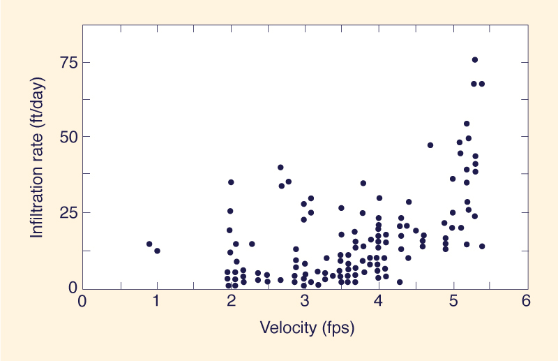
Baseline streambed infiltration rates along the mainstem Santa Cruz River and tributaries were qualitatively estimated based on the available literature.
Matlock (21) reported measurements of infiltration rates in the range of 2-10 ft/day along the main stem Santa Cruz from Continental to Cortaro and for Rillito Creek.
He also documented a tendency for the streambed infiltration rates to increase with flow velocity (largely because of the higher heads usually associated with higher velocities and stages), and measured infiltration rates as high as 76 ft/day, although most of them were below 25 ft/day (Fig. 7).
Lane (19) echoed Matlock in reporting streambed infiltration rates for the Santa Cruz River and tributaries in the range of 0.5-5.5 ft/day.
|
Fig. 7 Infiltration rate versus flow velocity (21).
|
Maps of the depth to water table were used to provide information for the initial assessment of streambed infiltration rates.
Values of 1, 2 and 4 ft/day were chosen as low, medium and high levels, respectively, for the base line set.
These values were later adjusted during the calibration phase to more closely reflect the actual magnitude of the streambed infiltration processes.
Rainfall Data
Rainfall data for the calibration phase (hindcast of the October 1983 flood) were assembled from various sources, including the following local, state and federal agencies: National Oceanic and Atmospheric Administration, National Weather Service; U.S. Forest Service; U.S. Bureau of Reclamation; University of Arizona, Water Resources Research Center; and Pima County Department of Transportation and Flood Control District, Tucson, Arizona.
Rainfall data for 31 stations, for the period of September 28-October 3, 1983, were assembled in suitable form.
The stations are spatially distributed throughout the basin, although station density is somewhat higher in the Tucson vicinity.
Data for 21 of these stations were hourly, and daily for the remaining ones.
Point rainfall depths for the general and local simulations were obtained from the pertinent NOAA NWS references (34,47).
This indicated that the 100-yr frequency 24-, 48- and 96-hr storms for the study region are approximately 4.6, 6.0 and 6.7 in., respectively. These values were reduced to account for depth-area correction following
Fig. 3 (34) and Fig. 4 (47).
8. STUDY RESULTS
Spatial and Temporal Resolution
Calibration, general and local storm runs were performed using a time interval of 7.5 min.
This was judged adequate to satisfy the lag requirements of the smaller subwatershed units.
A maximum subreach length of 1 mile was chosen to match the 7.5-min time interval and to guarantee the numerical consistency of stream channel routing (33).
The 1-mile upper limit on the subreach length triggered the automatic model generation of several additional subreach cross sections (resembling the input cross sections) up to 10 cross sections per reach in certain cases.
Calibration Runs
The objective of the calibration phase is to determine realistic levels of runoff curve numbers and streambed infiltration rates.
This is accomplished by adjusting the baseline values to match calculated and recorded flows.
To this end, the following values released by the Tucson office of the U.S. Geological Survey were used: (1) Continental, 45,000 cfs (1,274 m3/s); (2) Congress, 52,700 cfs (1,491 m3/s); (3) Cortaro, 65,000 cfs (1,840 m3/s); and (4) Rillito Creek (Tucson), 29,700 cfs (841 m3/s).
The Continental and Congress values were judged to be an overall higher reliability than the Cortaro and Rillito values (the latter were estimated by USGS using indirect means).
Accordingly, the calibration focused primarily on the Continental and Congress gages.
Stream gaging records (provisional discharges) furnished by USGS were
used as far as possible in verifying the accuracy in timing and shape of the calculated flood hydrographs.
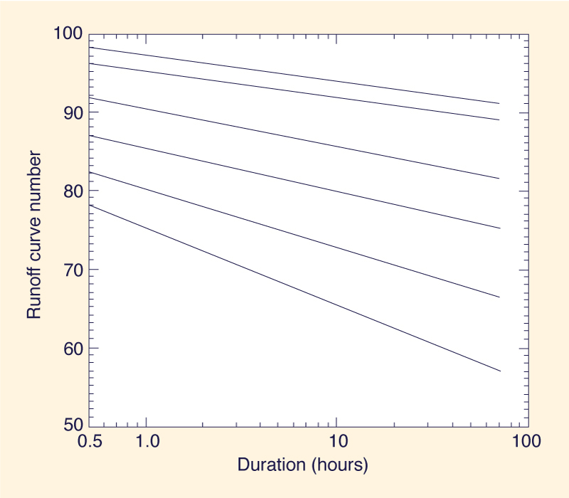
Calibration runs showed the need for the downward adjustment of runoff curve numbers and upward adjustment of streambed infiltration rates.
The reduction in runoff curve numbers was deemed justified in view of the basin size and corresponding rainfall durations (24, 48 and 96 hr).
Woodward (51) showed that baseline runoff curve numbers are most accurate for storm durations of up to 1 hr.
For storms lasting up to 72 hr, he proposed a downward adjustment of runoff curve numbers, as shown in Fig. 8.
Based on this figure, the baseline runoff curve numbers were reduced by an average of 10.
This led to runoff curve numbers in the range of 62-85, with a median of 76.
|
Fig. 8 Reduction in runoff curve numbers
with rainfall duration (51).
|
An increase in streambed infiltration rates was necessary to ensure a match of peak flows and runoff volumes for the October, 1983, flood data.
As pointed out by Matlock (21), flood stages lead to increased streambed infiltration rates and a subsequent loss of streamflow volume to groundwater reservoirs (14, 42, 50).
Accordingly, baseline infiltration rates were multiplied by 1.6 upstream of Continental, by 2.2 downstream of Continental but upstream of Congress, and by 5.2 downstream of Congress but upstream of Cortaro,
including the Rillito and Cañada del Oro tributaries).
This led to streambed infiltration rates in the range of 1.6-20.8 ft/day,
largely echoing Matlock's findings (Fig. 7).
With the aforementioned parameter adjustments, peak flows obtained during the calibration phase were:
(1) Continental, 44,500 cfs (1,259 m3/s); (2) Congress, 56,900 cfs (1,610 m3/s); (3) Cortaro, 83,900 cfs (2,374 m3/s); and (4) Rillito (Tucson), 26,200 cfs (741 m3/s).
General Storm Simulations
Results of the general storm simulations are summarized in Table 1.
This table shows the calculated peak flows at the Continental, Congress and Cortaro gages, for 24-, 48- and 96-hr storm durations.
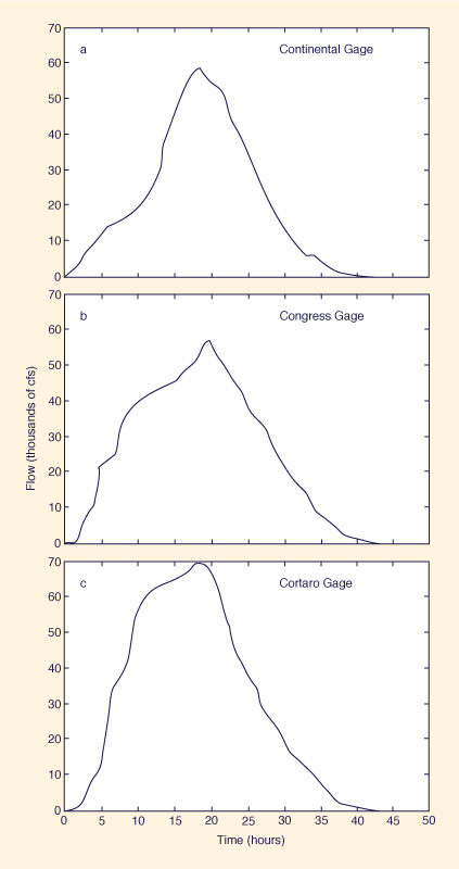
Figure 9 shows calculated hydrographs corresponding to the 24-hr general storm simulations at Continental, Congress and Cortaro.
Table 1. Summary of general storm simulations, 100-yr frequency.
|
Duration (hr)
(1) |
Peak Flow (cfs) |
Continental
(2) |
Congress
(3) |
Cortaro
(4) |
| 24 |
58,700 |
45,600 |
55,600 |
| 48 |
40,000 |
41,000 |
49,700 |
| 96 |
16,000 |
17,800 |
19,600 |
|
Note: 1 cfs = 0.0283 m3/s. |
|
|
Fig. 9 General storm simulated hydrographs.
|
Local Storm Simulations
Results of the local storm simulations are summarized in Table 2.
This table shows the calculated peak flows at the Continental,
Congress and Cortaro gages, for 24-, 48- and 96-hr storm
durations.
Table 2. Summary of local storm simulations, 100-yr frequency.
|
Duration (hr)
(1) |
Peak Flow (cfs) |
Continental
(2) |
Congress
(3) |
Cortaro
(4) |
| 24 |
41,500 |
58,600 |
38,100 |
| 48 |
47,200 |
67,000 |
47,800 |
| 96 |
35,900 |
46,800 |
35,400 |
|
Note: 1 cfs = 0.0283 m3/s. |
|
The area of coverage of each storm cell is described in Table 3.
These cells were chosen to maximize the calculated peak flows at the three locations.
All three cells are positioned immediately upstream of the gages.
Cell No. 3 was positioned on the mainstem Santa Cruz rather than on the Rillito or Cañada del Oro tributaries.
This is because the latter have higher streambed infiltration rates, resulting in generally lower peak flows.
Table 3. Description of cells used in local storm simulations.
|
Cell number
(1) |
Area
(square miles)
(2) |
Description
(3) |
Location
(4) |
| 1. Upstream of Continental gage |
429.9 |
Mainstem Santa Cruz River, Esperanza Wash, Madera Canyon Wash, Sopori Wash, Proctor Wash Batamote Wash, Sardina Canyon Wash, Papalote Wash, Montosa Canyon Wash and Cottonwood Canyon Wash |
Reach Subwatersheds:
21001,21101, 21201, 21301,31201,31301, 31401, 31402, 31403, 31404, 31405, 31501, 31601, 40112, 40113, 40114, 40115, 40116
Upland Subwatersheds:
17, 18, 19, 20, 46, 47, 48, 49, 50 |
| 2. Upstream of Congress gage |
414.5 |
Mainstem Santa Cruz River, Old West Branch, Julian Wash, Rodeo Wash, New West Branch, Franco Wash, and Sycamore Canyon Wash |
Reach Subwatersheds:
31801, 31901, 32001, 332101, 32201, 32301, 40118, 40119, 40120, 40121, 40122, 40123
Upland Subwatersheds:
54, 55, 56, 57 |
| 3. Upstream of Cortaro gage |
402.7 |
Mainstem Santa Cruz River, Old West Branch, Julian Wash, Rodeo Wash, New West Branch, and Franco Wash |
Reach Subwatersheds:
31901, ,32001, 32101, 32201, 32301, 40118, 40119, 40120, 40121, 40122, 40123, 40124, 40125, 40126
Upland Subwatersheds:
54, 55, 56, 57 |
| Note: See Fig. 6 for location of upland and reach subwatersheds. |
|
9. SANTA CRUZ RIVER REVISED DISCHARGES
The foregoing findings led Pima County Department of Transportation and Flood Control District to adopt revised discharges along the Santa Cruz River.
Effective January 1, 1985, the department set the regulatory and design discharges shown in Table 4.
The regulatory discharges are to be used for floodplain delineation and floodplain management, and the design discharges are to be used for channel and bridge improvement projects.
The values adopted reflect the calculated critical peak flow at Continental (general 24-hr storm) and critical peak flow at Congress (local 48-hr storm).
The Cortaro value was based on the result of the calibration phase, which showed a peak flow of 83,900 cfs for the October 1983 flood.
Table 4. Regulatory and design discharges.
|
Location
(1) |
Discharges (cfs) |
Regulatory
(2) |
Design
(3) |
| Continental |
45,000 |
55,000 |
| Congress |
60,000 |
70,000 |
| Cortaro |
70,000 |
80,000 |
|
10. COMPARISON WITH OTHER REGIONAL FLOOD ESTIMATES
A comparison with other regional flood estimates appears justified. Roeske (41) developed a method for estimating regional flood frequencies in six regions in Arizona.
Roeske's region No. 5 covers southeastern Arizona and encompasses the Santa Cruz basin.
Roeske's region No. 5 equation is the following:
in which Q100 = is the 100-yr frequency flood discharge, in cubic feet per second, and A = the basin drainage area, in square miles.
Reich et al. (40) developed a regional estimate for Q100 using data for the ARS Walnut Gulch Experimental Watershed in southeastern Arizona.
The equation of Reich et al. is the following:
| Q100 = 2,360 A 0.688 - 0.128 logA
| (2) |
which is strictly applicable to drainage areas in the range of 1,613 square miles.
For the larger areas of this study, the equation of Reich et al. would predict comparatively low values.
Malvick (20) analyzed 3,604 station years of data from 151 gaging stations throughout Arizona to produce a net of regional flood frequency values for a range of watershed/basin sizes from 0.01 to 100,000 square miles.
Malvick's equation for Q100 is the following:
| Q100 = 826 A 0.789 - 0.067 logA
| (3) |
By shifting Malvick's curve sideways from right to left about half a log cycle, Boughton and Renard (2)
were able to produce a regional envelope curve encompassing most of the earlier regional studies.
Boughton and Renard's equation is the following:
| Q100 = 2,200 A 0.736 - 0.082 logA
| (4) |
For comparison purposes, Eqs. 1, 3 and 4 are applied to the Continental (1,682 square miles), Congress
(2,222 square miles), and Cortaro (3,503 square miles) gages.
The calculated Q100 values are shown in Table 5, with the values adopted by Pima County on the basis of this study's findings.
Table 5. Comparison with regional flood estimates, Santa Cruz basin (peak flow, in cfs).
|
Gage
(1) |
Adopted by Pima County |
Boughton and Renard
(Ref. 2)
(4) |
Malvick
(Ref. 20)
(5) |
Roeske
(Ref. 41)
(6) |
Regulatory
(2) |
Design
(3) |
| Continental |
45,000 |
55,000 |
73,000 |
58,000 |
34,000 |
| Congress |
60,000 |
70,000 |
77,000 |
64,000 |
39,000 |
| Cortaro |
70,000 |
80,000 |
83,000 |
74,000 |
47,000 |
|
11. SUMMARY AND CONCLUSIONS
A hydrologic evaluation of the Santa Cruz River basin upstream of Cortaro Farms Bridge near Tucson, Arizona, is documented herein.
The evaluation uses novel techniques of deterministic hydrologic modeling in a computer-based, data-intensive environment to calculate frequency-based floods at proposed bridge improvement sites.
A comprehensive computer modeling system, capable of simultaneously handling the complex topology of the entire basin, is driven by 100-yr frequency NWS rainfall events of 24-, 48- and 96-hr durations.
Model calibration is accomplished by hindcasting the flood of October 1983, which produced record flows throughout southeastern Arizona.
Once calibrated, a series of general and local storms are simulated by the model.
General storms cover the entire basin with low-intensity rainfall events; local storms cover selected portions of the basin with high-intensity rainfall events.
Critical peak flows are shown to be associated with a combination of general 24-hr and local 98-hr storms.
The results of the simulation led Pima County to adopt revised flood discharges along the Santa Cruz River.
These values are used for flood plain delineation and management, and channel and bridge improvement and design.
ACKNOWLEDGMENTS
This study was supported by the Pima County Department of Transportation and Flood Control District, Tucson, Arizona, Charles H. Huckleberry, Director.
APPENDIX. REFERENCES
"Arizona Weather Summary. 1983. "Office of the State Climatologist for Arizona," Vol. 10, No. 4, Oct., 1983, and No. 5, Nov.
Boughton, W. C., and K. G. Renard. 1984. "Flood Frequency Characteristics of Some Arizona Watersheds," Water Resources Bulletin. AWRA, Vol. 2D, No. 5, Oct., 761-769.
Boyer, D. G., and E. I. De Cook. 1976. 'The Effect of an Intensive Summer Thunderstorm on a Semiarid Urbanized Watershed," Proceedings of the April 29-May 1, 1976, Meeting of the Arizona Section, AWRA, and the Hydrology Section, Arizona Academy of Science, held at Tucson, Ariz.
Burkham, D. F. "Depletion of Streamflow by Infiltration in the Main Channels of the Tucson Basin, Southeastern Arizona," Water Supply Paper 1939- B, U.S. Geological Survey.
Cecilio, C. B. 1984. Discussion of "Conservatism of Probable Maximum Flood Estimates," by Bi-Huei Wang and Russell W. Revell, Journal of Hydraulic Engineering, ASCE, Vol. 110, No. 4, April, 545-546.
"Climatological Data, Arizona." 1983. Vol. 87, Nos. 9 and 10, U.S. Department of Commerce, National Oceanic and Atmospheric Administration, National Weather Service, Sept. and Oct.
"Computer Program for Project Formulation-Hydrology," 1982. Technical Release Number 20, USDA Soil Conservation Service, Engineering Division, Washington, D.C., Draft, May.
Conde de la Torre, A., "Streamflow in the Upper Santa Cruz River Basin, Santa Cruz and Pima Counties, Arizona," Water Supply Paper 1939-A, U.S. Geological Survey.
"Depth-Area Ratios in the Semiarid Southwest United States." 1984. NOAA Technical Memorandum NWS HYDRO-40, U.S. Department of Commerce, Silver Spring, Md., Aug.
"Flood Hazard Information, Santa Cruz River, Santa Cruz County, Arizona." 1971.
U.S. Army Corps of Engineers, Jan.
"Flood Hazard Information, Santa Cruz River, Vicinity of Sonoita Creek Confluence." 1969.
U.S. Army Corps of Engineers, Nov.
"Flood Insurance Study." 1982. Federal Emergency Management Agency, Pima County, Ariz., Dec., 1982.
"Flood Insurance Study." 1980. Federal Emergency Management Agency, Santa Cruz County, Ariz., Feb.
"Groundwater in the Santa Cruz Valley, Arizona." 1972. Technical Bulletin 194, University of Arizona, Agricultural Experiment Station, Tucson, Ariz., April.
"HEC-1, Flood Hydrograph Package, User's Manual." 1981. U.S. Army Corps of Engineers, Hydrologic Engineering Center, Davis, Calif.
"Interduration Precipitation Relations for Storms-Western United States." 1981.
Technical Report NWS 27, U.S. Department of Commerce, National Oceanic and Atmospheric Administration, National Weather Service, Office of Hydrology, Silver Spring, Md., Sept.
"Interim Report, Probable Maximum Precipitation in California." 1961. NOAA Hydrometeorological Report No. 36, U.S. Department of Commerce, Oct. (reprinted with revisions of Oct., 1969).
Keppel, R. V., and K. G. Renard. 1962., 'Transmission Losses in Ephemeral Stream Beds," Journal of the Hydraulics Division, ASCE, Vol. 88, No. HY3, March.
Lane, L. J. 1983. "Chapter 19: Transmission Losses," USDA Soil Conservation Service National Engineering Handbook, Section 4, April.
Malvick, A. J. 1980. "A Magnitude-Frequency-Area Relation for Floods in Arizona," Research Report No. 2, Engineering Experiment Station, College of Engineering, University of Arizona, Tucson, Ariz., 186 pages.
Matlock, W. G. 1965. 'The Effect of Silt-Laden Water on Infiltration in Alluvial Channels," dissertation presented to the University of Arizona, at Tucson, Ariz., in 1965, in partial fulfillment of the requirements for the degree of Doctor of Philosophy.
McCuen, R. H., W. J. Rawls, and S. L. Wong, 1984. "SCS Urban Peak Flow Methods," Journal of Hydraulic Engineering, ASCE, Vol. 110, No. 3, March, 290-299.
"National Engineering Handbook, Section 4: Hydrology (NEH4). 1973.
USDA Sod Conservation Service," Washington, D.C.
Osborn, H. B., L. J. Lane, and V. A. Myers. 1980, "Rainfall-Watershed Relationships for Southwestern Thunderstorms," ASAE Transactions, Vol. 23, No. 1, 82-87, and 91.
Osborn, H. B., E. D. Shirley, D. R. Davis, and R. B. Koehler. 1980. "Model of Time and Space Distribution of Rainfall in Arizona and New Mexico," ARM-W-14, USDA Science and Education Administration, May.
Osborn, H. B., and L. J. Lane. 1981. "Point-Area Frequency Conversions for Summer Rainfall in Southeastern Arizona," Proceedings of the May 1-2,1981, Meetings of the Arizona Section, AWRA, and the Hydrology Section, Arizona-Nevada Academy of Sciences, held at Tucson, Arizona.
Osborn, H. B. 1981. "Quantifiable Differences Between Airmass and Frontal-Convective Thunderstorm Rainfall in the Southwestern United States," Proceedings, May 18-21, 1981, International Symposium on Rainfall-Runoff Model-ing, Mississippi State University, Mississippi State, Miss.
Osborn, H. B. 1983. "Timing and Duration of High Rainfall Rates in the South-western United States," Water Resources Research, Vol. 19, No. 4, Aug., 1036-1042.
Osborn, H. B. 1983. 'Precipitation Characteristics Affecting Hydrologic Response of Southwestern Rangelands," ARM-W-34, USDA Agricultural Research Service, Jan.
Ponce, V. M., and D. B. Simons, 1977. "Shallow Wave Propagation in Open Channel Flow," Journal of the Hydraulics Division, ASCE, Vol. 103, No. HY12, Dec., 1461-1476.
Ponce, V. M., and V. Yevjevich. 1978. "Muskingum-Cunge Method with Variable Parameters," Journal of the Hydraulics Division, ASCE, Vol. 104, No. HY12, Dec., 1663-1667.
Ponce, V. M. 1979. "A Simplified Muskingum Routing Equation," Journal of the Hydraulics Division, ASCE, Vol. 105, No. HY1, Jan., 85-91.
Ponce, V. M., and F. D. Theurer. "Accuracy Criteria in Diffusion Routing," Journal of the Hydraulics Division, ASCE, Vol. 108, No. HY6, June, 747-757.
"Precipitation Atlas of the Western United States. 1973. Vol. VII-Arizona," U.S. Department of Commerce, National Oceanic and Atmospheric Administration.
"Probable Maximum Precipitation, Colorado River and Great Basin Drainage." 1977. NOAA Hydrometeorological Report No. 49, U.S. Department of Commerce, Sept.
"Probable Maximum Precipitation Estimates, United States Between the Continental Divide
and the 103rd Meridian." 1984. NOAA Hydrometeorological Report No. 55, U.S.
Department of Commerce, March.
"Probable Maximum Precipitation Estimates, United States East of the 105th Meridian." 1978.
NOAA Hydrometeorological Report No. 51, U.S. Department of Commerce, June.
"Probable Maximum Precipitation in the Hawaiian Islands." 1963. NOAA Hydrometeorological Report No. 39, U.S. Department of Commerce.
"Probable Maximum Precipitation, Northwest States." 1966. NOAA Hydrometeorological Report No. 43, U.S. Department of Commerce, November, 1966.
Reich, B. M., H. B. Osborn, and M. C. Baker "Tests on Arizona's New Flood Estimates," Hydrology and Water Resources in Arizona and the Southwest, Vol. 9, University of Arizona, Tucson, Ariz., 65-74.
Roeske, R. H. 1978. "Methods for Estimating the Magnitude and Frequency of Floods in Arizona" Final Report ADOT-RS-15-121, U.S. Geological Survey, Tucson, Adz., 82 pages.
"Santa Cruz-San Pedro River Basin, Arizona: Resource Inventory." 1977. USDA Soil Conservation Service, Economic Research Service, Forest Service, in cooperation with the Arizona Water Commission, Aug.
Simanton, J. R., K. G. Renard, and N. G. Sutter. 1973.
"Procedure for Identifying Parameters Affecting Storm Runoff Volumes in a Semiarid Environment," ARS-W-1, USDA Agricultural Research Service, Western Region, Jan.
"Soil Survey of Santa Cruz and Parts of Cochise and Pima Counties, Arizona." 1979. USDA Soil Conservation Service and Forest Service, in cooperation with University of Arizona Agricultural Experiment Station, April.
"Soil Survey of Tucson-Avra Valley Area, Arizona." 1972. USDA Soil Conservation Service, in cooperation with the University of Arizona Agricultural Experiment Station, April.
"Statistical Summaries of Arizona Streamflow Data." 1979. USGS Water Resources Investigations 79-5, U.S. Department of the interior, Geological Survey, Jan.
"Two-to-Ten Day Precipitation for Return Periods of 2 to 100 Years in the Contiguous United States." 1964.
U.S. Weather Bureau Technical Paper No. 49, U.S. Department of Commerce.
"Water Data Report, Arizona, 81-1," U.S. Department of the Interior, Geological Survey.
"Water Resources Data, Arizona, Water Year 1981," U.S. Department of the Interior, Geological Survey.
Wilson, L. G., K. J. De Cook, and S. P. , Neuman, 1980. "Regional Recharge Research for Southwest Alluvial Basins," Water Resources Research Center, Department of Hydrology and Water Resources,
University of Arizona, Tucson, Ariz.
Woodward, D. 1973. "Runoff Curve Numbers for Semiarid Range and Forest Conditions,"
Paper 73-209, presented at the June 17-20, 1973,
Annual Meeting of the American Society of Agricultural Engineers, held at Lexington, Ky.
|