|
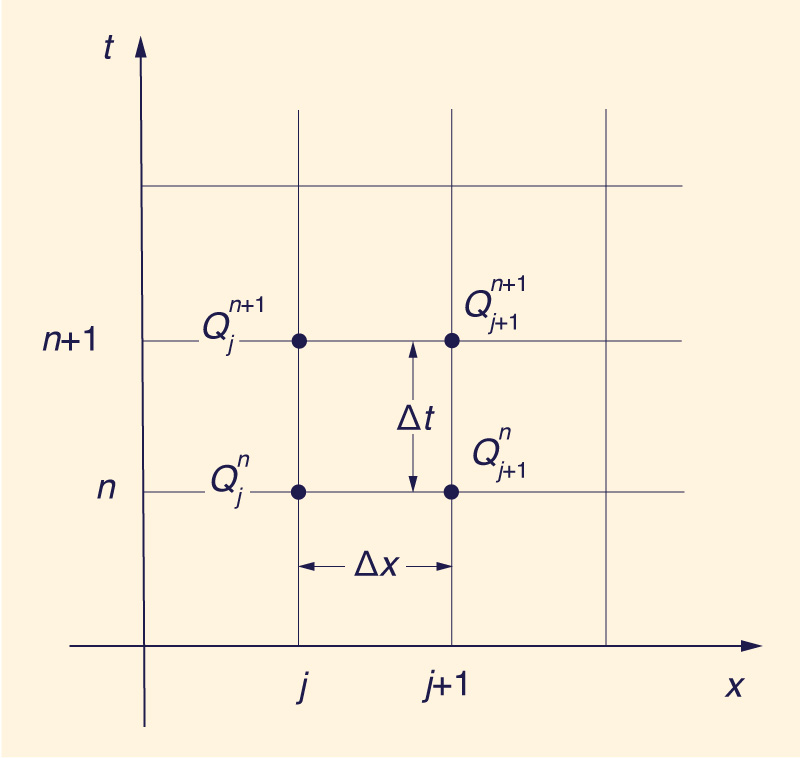
FIG. 1. - Space-time discretization in Muskingum method.
Taking the time derivative at the downstream section is tantamount to an assumption of reservoir-type storage. Therefore, in discrete solutions, the assumption of a linear reservoir provides the mechanism by which numerical diffusion is introduced in the computations in order to simulate the physical diffusion processes in the watershed environment.
The extension of the numerical diffusion effect to the concept of a cascade of linear reservoirs is readily envisaged. In doing so, a second parameter, n, is introduced; n represents the number of reservoirs in series. Such a two-parameter model, {K, n}, increases the flexibility of the simulation process while staying within the computational framework established by the one-parameter model.
2. KINEMATIC WAVE ROUTING AND NUMERICAL DIFFUSION
Cunge (2) pioneered in establishing the role of numerical diffusion in connection with kinematic wave routing. He reasoned that since the linear kinematic wave equation is an equation of pure convection, the diffusion calculated by a numerical scheme based on this equation had to originate in the scheme itself. He traced the origin of this numerical diffusion effect to the truncation errors arising from "off-centering" the temporal derivative term. This led to an improved understanding of kinematic wave routing techniques, among which the Muskingum method is a notable example. For the sake of completeness, the development of the Muskingum-Cunge method is briefly reviewed herein.
The kinematic wave equation is of the form:
∂Q ∂Q
_____ + c _____ = 0
∂t ∂x
| (3) |
in which Q = discharge; c = kinematic wave celerity; t = time variable; and x = space variable. The kinematic wave celerity is either taken as constant (linear case) or varied with the flow (quasilinear case) (4, 6, 8). In the linear case, the discretization of Eq. 3 on the x-t plane (Fig. 1) leads to the well-known Muskingum formula (1):
|
Q j+1 n+1 = C1Q j n + C2 Q j n+1 + C3 Q j+1 n
| (4) |
in which C1, C2 and C3 are coefficients defined as follows:
Δt
______ + 2X
K
C1 = _______________________
Δt
______ + 2 ( 1 - X )
K
| (5) |
Δt
______ - 2X
K
C2 = _______________________
Δt
______ + 2 ( 1 - X )
K
| (6) |
Δt
2 ( 1 - X ) - ______
K
C3 = _______________________
Δt
______ + 2 ( 1 - X )
K
| (7) |
in which Δx = reach length; Δt = routing interval; K = travel time (K = Δx /c); and X = weighting factor of the temporal derivative term.
An estimate of the value of X can be obtained by matching the numerical diffusion coefficient of the discretized kinematic wave equation with the physical diffusion coefficient of the convection-diffusion equation
(the diffusion wave equation). This leads to:
1 q
X = ___ ( 1 - __________ )
2 So c Δx
| (8) |
in which q = unit-width discharge; and So = average channel bed slope.
A convenient form of expressing the coefficients of Eqs. 5-7 is in terms of the Courant and cell Reynolds numbers. The Courant number is defined as follows:
and the cell Reynolds number as follows:
q
D = __________
So c Δx
| (10) |
leading to:
1 + C - D
C1 = _____________
1 + C + D
| (11) |
- 1 + C + D
C2 = _____________
1 + C + D
| (12) |
1 - C + D
C3 = _____________
1 + C + D
| (13) |
3. CLASSICAL APPROACH TO MUSKINGUM METHOD
The classical approach to the derivation of the Muskingum method utilizes the equation of continuity in its spatially integrated form:
dV
I - O = ______
dt
| (14) |
in which I = inflow; O = outflow; and V = reach storage. Furthermore, a weighted funcion of inflow, outflow, and storage of the form:
V = K [XI + ( 1 - X )O ]
| (15) |
is used in lieu of the momentum equation.
The solution of Eqs. 14 and 15 in the discrete x - t plane leads to the same Eq. 4 which was obtained from the kinematic wave equation, Eq. 3. The kinematic wave equation is derived from the continuity equation and a simplified form of the momentum equation that considers only the balance of
gravitational and frictional forces, such that:
in which Sf = friction slope. Therefore, it follows that Eq. 15 is an analog of Eq. 16 rather than an analog of the full momentum equation.
4. LINEAR RESERVOIRS
The concept of linear reservoirs has been widely used in connection with the mathematical modeling of surface runoff. It is the major building block of the SSARR model (9),
which uses it in both its watershed and stream channel routing components. The Kalinin-Milyukov method of flood routing (4), developed in the Soviet Union, is another method
whose development closely parallels that of the linear reservoir concept. Interestingly enough, in stream channel routing, the assumption of a linear reservoir (Eq. 1) leads
to the so-called "characteristic reach length," as in the Kalinin-Milyukov method and similar more recent developments (7). The characteristic reach length Δxc
is calculated by making X = 0 in Eq. 8:
q
Δxc = _______
So c
| (17) |
The idea of a characteristic reach length associated with stream channel routing is not readily transposable
to watershed routing. The complexity of the watershed environment precludes the estimation of Δxc
on the basis of measurable physical quantities. Therefore, while the linear reservoir concept can be applied to stream
channel routing in a predictive sense, it can only be applied to watershed routing in the identification sense.
5. SSARR ROUTING EQUATION
The SSARR routing equation is a particular case of the Muskingum method in which the concept of reservoir-type storage is implemented by setting X = 0 (4). From Eqs. 8 and 10, X = 0 implies that D = 1. Substituting D = 1 in Eqs. 11 to 13 leads to:
C
C1 = C2 = _________
2 + C
| (18) |
and:
2 - C
C3 = ________
2 + C
| (19) |
Substituting Eqs. 18 and 19 into Eq. 4 gives:
2C Qjn + Qjn+1 2 - C
Qj+1n+1 = (________) (_______________) + (___________) Qj+1n
2 + C 2 2 + C
| (20) |
or by rearrangement:
2C Qjn + Qjn+1
Qj+1n+1 = (________) [(______________) - Qj+1n ] + Qj+1n
2 + C 2
| (21) |
which is recognized as the SSARR routing equation (since C = c Δt / Δx = Δt / K = Δt / Ts).
6. CASCADE OF LINEAR RESERVOIRS
Equation 21 is used in the numerical model of a cascade of linear reservoirs such as the SSARR model. A close examination of Eq. 21 leads to the following conclusions:
For C = 2 (i.e., the routing interval is twice the time of storage), the outflow is equal to the average inflow;
For C > 2 (i.e., the routing interval exceeds twice the time of storage), there is a numerical amplification effect; and
For 0 < C < 2 (i.e., the routing interval ts smaller than twice the time of storage), there is a numerical diffusion effect. Note that the amount of diffusion is a function of the Courant number, smaller values of C resulting in a larger diffusion effect.
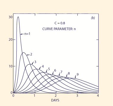
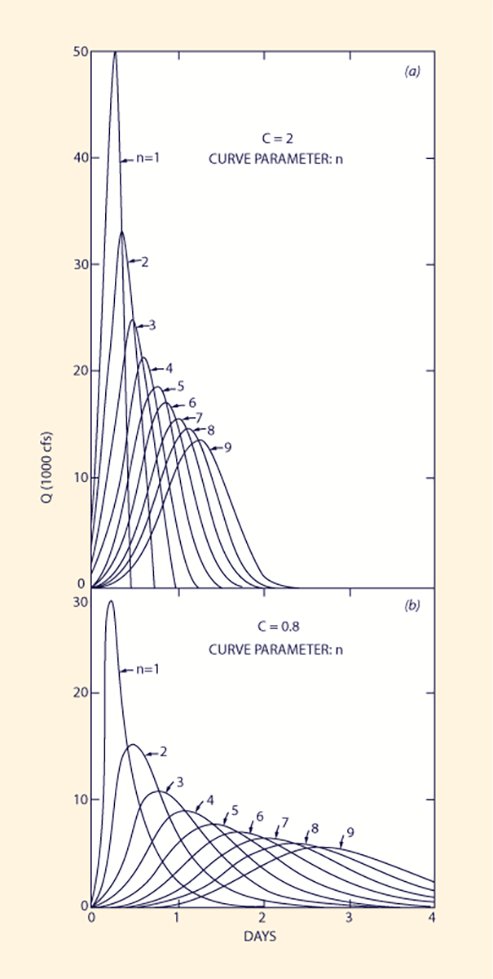
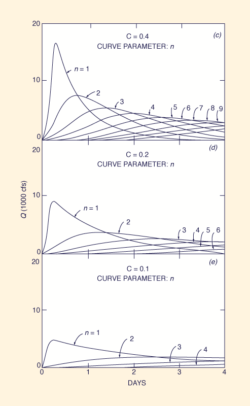
FIG. 2. - Computed hydrographs as function of Courant number C and number of linear reservoirs in series n:
(a) C = 2.0; (b) C = 0.8; (c) C = 0.4; (d) C = 0.2; (e) C = 0.1.
The flexibility of the conceptual model of a cascade of linear reservoirs to model a wide range of watershed runoff events is illustrated by applying Eq. 21 to an individual 1-in. 6-h storm uniformly distributed over an area of 465 sq miles (1,204 km2), corresponding to an inflow of 50,000 cfs (1,416 m2/s). Fig. 2 shows the computed hydrographs that result for a cascade of up to nine linear reservoirs, for Courant numbers of 2.0, 0.8, 0.4, 0.2, and 0.1. The examination of this figure enables the following conclusions to be drawn:
For a given Courant number, a greater number of linear reservoirs results in smaller peak flows and longer delay times.
For a given number of reservoirs, smaller values of the Courant number result in smaller peak flows and longer delay times.
The hydrograph skewness is a function of the Courant number. As the Courant number increases, the positive skewness effect (fast rise, slow fall) decreases. As the Courant number tends to the value C = 2, the skewness vanishes.
The integration of the area under the computed hydrographs shows that the method is mass conservative. No appreciable gains or losses of mass have been detected.
7. SUMMARY AND CONCLUSIONS
The conceptual model of a cascade of linear reservoirs, in particular the SSARR routing equation, is reviewed in the light of the theory of numerical diffusion. The SSARR routing equation is shown to be a special case of the Muskingum routing equation. Since the latter simulates the diffusion processes by "off-centering" the temporal derivative in its discrete formulation, it follows that the same numerical diffusion mechanism underlies the SSARR routing equation and its associated linear reservoir assumption. The extension of the technique to a cascade of linear reservoirs, thus providing an additional parameter for simulation purposes, is readily envisioned.
In practice, the use of a conceptual model such as the cascade of linear reservoirs remains a problem of system identification: Given an excitation (excess rainfall) and system response (basin outflow), the overall system characteristics (model parameters) are sought by calibration. In the case of the SSARR routing equation, the model parameters are the Courant number, C, and the number of reservoirs, n. Once the parameters are determined, it is hoped that they can be used in the predictive stages of modeling. To the extent that this can be done, at least approximately (3, 10), the model retains an essentially linear structure.
APENDIX I. - REFERENCES
-
Chow, V. T., Handbook of applied hydrology, McGraw-Hill Book Co., Inc., New York, N.Y., 1974.
-
Cunge, J, A. 1969. "On the subject of a flood propagation computation method (Muskingum method)," Journal of Hydraulic Research, Vol. 7, No. 2, 205-230.
-
Dodge, J. C. I. 1977. "Problems and methods of Rainfall-Runoff modeling," Mathematical Models for Surface Water Hydrology, T. A. Ciriani, V. Maione and J. R. Wallis, eds., John Wiley and Sons, London, England.
-
Miller, W. A., and J. A. Cunge, J. A. 1975."Simplified equations of unsteady flow," Unsteady Flow in Open Channels, K. Mahmood and V. Yevjevich, eds., Water Resources Publication,
Fort Collins, Colo., 183-257.
-
Nash, J. E. 1957. "On the norm of the instantaneous unit hydrograph," International Association for Scientific Hydrology, Publication No. 45, Vol. 3, 110.121.
-
Ponce, V. M., and V. Yevjevich, V. 1978. "The Muskingum-Cunge method with variable parameters," Journal of the Hydraulics Division, ASCE, Vol. 104, No. HY12, Proc. Paper 14199, Dec.
-
Ponce, V. M. 1979. "Simplified Muskingum routing equation," Journal of the Hydraulics Division, ASCE, Vol. 105, No. HY1, Proc. Paper 14275, Jan., 85-91.
-
Price, R. K. 1978. "A river catchment flood model," Proceedings of the Institution of Civil Engineers, London, England, Part 2, Vol. 65, Sept., 655-688.
-
Program Description and User Manual for SSARR Model, Streamflow Synthesis and Reservoir Regulation. 1972.
U.S. Army Engineer North Pacific Division, Portland, Oreg., Sept., revised June, 1975.
-
Rao, R. A., J. M. Delleur, and B. S. Sarma. 1972. "Conceptual hydrologic models for urbanizing basins." Journal of the Hydraulics Division, ASCE, Vol. 98, No. HY7, Proc. Paper 9024, July, 1205-1220.
-
"WMO project on intercomparison of conceptual models used in operational hydrological forecasting," 1977.
Mathematical Models for Surface Water Hydrology, T. A. Ciriani, V. Maione and J. R. Wallis, eds., John Wiley and Sons, London, England.
APENDIX II. NOTATION
The following symbols are used in this paper:
C = Courant number, Eq. 9;
C1, C2 and C3 = coefficients, Eqs. 5-7;
c = kinematic wave celerity;
D = cell Reynolds number, Eq. 10;
I = inflow;
K = storage coefficient, Muskingum parameter (travel time);
n = number of reservoirs, number of increments of storage;
0 = outflow;
Q = discharge;
q = unit-width discharge;
Sf = friction slope;
So = average channel bed slope;
Ts = time of storage;
t = time variable;
V = reach storage;
X = Muskingum parameter (weighting factor);
x = space variable;
Δx = reach length;
Δxc = characteristic reach length, Eq. 17;
Δt = routing interval; and
Γ(n) = gamma function of argument n.
Subscripts
j = space index; and
n = time index.
|