|
M1 water-surface profile. M1 WATER-SURFACE PROFILE CALCULATED ONLINE
Professor Emeritus of Civil and Environmental Engineering
San Diego State University, San Diego,
California
1. INTRODUCTION
A water-surface profile is a feature of
the hydraulics of open channels which describes the variation of the water-surface elevation in
the longitudinal direction (one dimension x in space),
under a steady equilibrium flow condition. There are twelve (12) types of water-surface profiles,
depending on the Froude number F and the ratio So /Sc , in which
So = bottom slope, and Sc = critical slope.
The critical slope Sc
is equal to 1/8 of the Darcy-Weisbach friction factor f.
Table 1 lists the twelve types of profiles (Ponce, 2014).
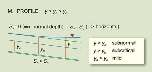
In this article, we describe the M1 water-surface profile, a retarded (backwater) subcritical/subnormal profile, which may well be the most common profile in practice. The M1 profile depicts flow in a mild channel, upstream of a reservoir (Fig. 1). We present two examples and show the respective online calculations.
Fig. 1 M1 water-surface profile.
2. GOVERNING EQUATION
Chow (1959) has presented the classical way of expressing the governing equation of steady, gradually varied flow.
A more cogent, dimensionless presentation, focusing on critical slope, has been
advanced by Ponce (2014) and is presented here.
In terms of critical slope, the general equation for flow-depth gradient dy/dx is:
in which So = channel (bottom) slope, Sc = critical slope,
P = wetted perimeter,
T = channel top width,
For (P / T ) = (Pc / Tc ), Eq. 1 reduces to:
For conciseness, the flow-depth gradient may be written as:
Substituting Eq. 3 into Eq. 2, the flow-depth gradient is:
Equation 2, or Equation 4, its reduced
form,
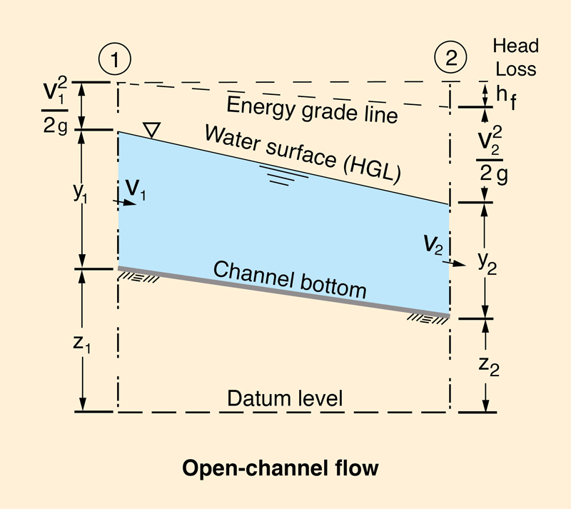
is the steady gradually varied flow equation (Fig. 2).
Fig. 2 Definition sketch for energy balance in open-channel flow.
3. ONLINE CALCULATION: EXAMPLE A
We pose an example of the calculation
of an M1 profile in a natural channel using the online calculator
ONLINE_WSPROFILES_21.
The following box shows the input data.
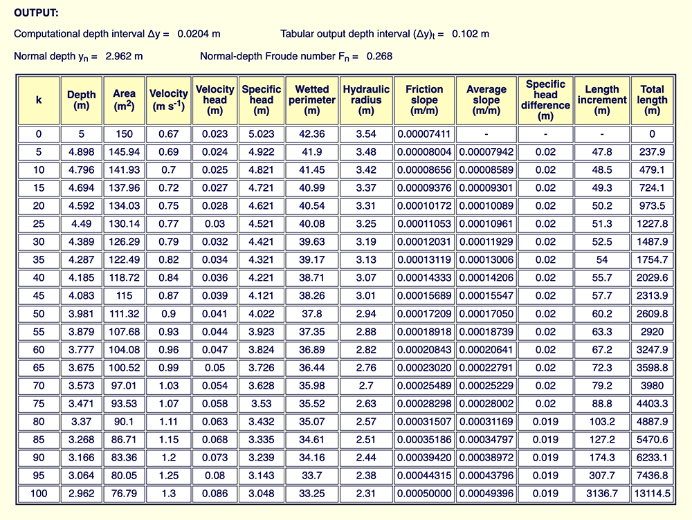
Output. The results show that the (flow) depth at the downstream boundary (yd = 5 m) will decrease gradually to the normal depth in the upstream end yn = 2.962 m. The total distance, from downstream boundary to upstream end, is: L = 13,114.5 m.
4. ONLINE CALCULATION: EXAMPLE B
We pose an example of the calculation
of an M1 profile in a lined channel using the online calculator
ONLINE_WSPROFILES_21.
The following box shows the input data.
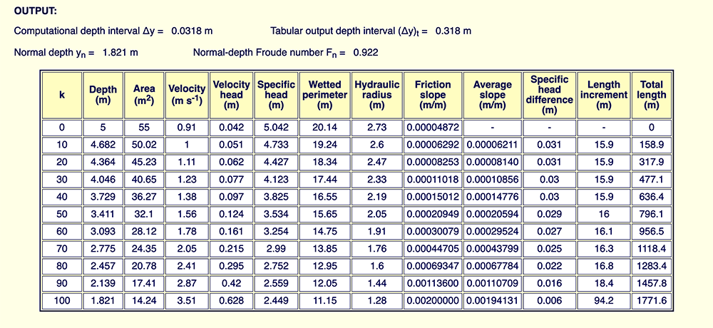
Output. The results show that the (flow) depth at the downstream boundary (yd = 5 m) will decrease gradually to the normal depth in the upstream end yn = 1.821 m. The total distance, from downstream boundary to upstream end, is: L = 1,771.6 m.
5. SUMMARY
An online calculation of an
M1 open-channel flow water-surface profile is shown in detail.
REFERENCES
Chow, V. T. 1959. Open-channel hydraulics. McGraw-Hill, Inc, New York, NY.
Ponce, V. M. 2014b.
Fundamentals of Open-channel Hydraulics.
Online textbook. | |||||||||||||||||||||||||||||||||||||||||||||||||||||||||||||||||||||||||||||||||||


| 231025 |