1. INTRODUCTION
Flow in an alluvial channel is of an unsteady nonuniform type. Accordingly, the water and sediment discharge vary in time and space. In an alluvial channel reach, equilibrium flows are defined as those in which the sediment inflow
and outflow are balanced over a sufficiently long period of time.
The study of bed transient propagation may be approached from an analytical or numerical standpoint. The analytical approach (4) may be used to study certain types of transients, but the simplifying assumptions are too strenuous for the general case. On the other hand, numerical models can usually be built using a smaller number of assumptions and are more versatile than analytical solutions in the specification of boundary conditions. Therefore, a numerical model is regarded as a more effective tool in the study of bed transient propagation. Relevant questions of stability, consistency, and convergence arise every time a numerical modeling project is attempted. Nevertheless, the experience with this type of modeling in the last two decades indicates that these difficulties can usually be brought under control.
A numerical model involves the solution of one or more governing partial differential equations by the use of finite difference techniques. In the bed transient
problem, there are three equations: A practical alternative to the sequential routing method for the cases in which the bed
transients are of primary interest is given by the known-discharge method. The rationale for this method of solution lies in the fact that the bed transients
propagate much slower pace than the water surface transients. Therefore, within one time step, a steady water discharge may be assumed to hold. The steady water discharge assumption dictates that the water continuity equation be described by a simple algebraic relation. Therefore, only two differential equations remain: (1) the sediment continuity equation; and (2) the equation of motion. Furthermore, the neglect of the local acceleration term of the equation of motion follows directly from the steady water discharge assumption. As with the flood routing models based on a kinematic formulation, the unsteady nature of the problem is preserved through the rate-of-change term in the continuity equation. The numerical solution of these two equations may be accomplished in two ways: (1) an uncoupled mode (5) may be used by first solving for the water surface profile and then adjusting the bed elevation using the sediment continuity equation; and (2) a coupled mode (3,8), by simultaneously solving the sediment continuity equation and the equation of motion. Uncoupled models are based on explicit schemes, while coupled models lend themselves to computation by implicit schemes. Therefore, the coupled models are more flexible, since the maximum size of the time step is not governed by the strict stability criterion usually associated with explicit schemes, but rather, its size is solely based on accuracy considerations.
A known-discharge coupled bed transient model is presented in this paper. The model represents an improvement over earlier models of the same type in that instability due to ill-posing of the bed material transport function (6) is circumvented, and errors in mass conservation due to improper formulation of the boundary condition (3) are avoided by use of a strictly nonlinear formulation.
Three limitations of the mathematical model are apparent at the outset. The one-dimensional formulation does not permit the description of meandering. Also, since no provision is made for the routing of sediment by size fractions, no account can be made of armoring phenomena. In addition, the transport function does not effectively account for the condition of incipient motion; therefore, the model would work best when the flow conditions are such that the Froude number is greater
The remainder of the present paper treats the following subjects in detail: (1) governing equations; (2) finite difference scheme; (3) boundary conditions; (4) stability and convergence; and
2. GOVERNING EQUATIONS
The governing equations, expressed per unit of channel width, are the continuity of sediment:
∂qs ∂ ∂z
1 ∂u ∂ u 2 ∂d ∂z
According to Mahmood and the first writer (8), in river flow the temporal concentration variation term in Eq. 1 is very small when compared with the remaining terms; therefore, it is neglected here.
∂qs ∂z
q 2 ∂ ∂d ∂z
Two supplementary equations are necessary in order to solve the system of Eqs. 3 and 4: (1) a flow resistance formula; and (2) a bed material transport formula. No closed form equation for either is available, although empirical equations have been used in the past with some success.
The resistance and transport functions used herein are the following:
For a wide channel, ƒr = f /8, in which f = the Darcy-Weisbach friction factor.
3. FINITE-DIFFERENCE SCHEME
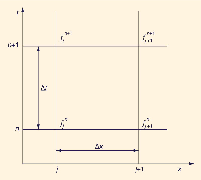
The four-point implicit scheme of Preissmann (6) is used here. The scheme is expressed by the following operators (refer to Fig. 1);
in which ƒ = a dependent variable, and θ = weighting factor of the implicit scheme.
The application of Eqs. 7-9 to Eqs. 3 and 4 in the discrete x - t plane yields a set of simultaneous nonlinear algebraic equations. In order to solve for the values of the dependent variables at the advanced time level without resorting to an iterative process, a linearization scheme is devised.
The linearization scheme is of the following form:
in which δ = a real number.
The solution of the system of simultaneous linear equations is accomplished by the well-known double sweep algorithm (6).
4. BOUNDARY CONDITIONS
At the upstream boundary, either the change in stage or bed elevation with time may be specified. Alternatively, the flow depth can be specified. This enables the modeling of a nonequilibrium sediment inflow hydrograph by relating the change in flow depth to the change in sediment inflow. For varying water and sediment discharge, the upstream boundary condition is formulated as follows (7):
in which ∆d1T = change in flow depth at the
upstream boundary; ∆d1S = change in flow depth
at the upstream boundary due to nonequilibrium sediment inflow;
and ∆d1Q = change in flow depth at the upstream boundary due to nonequilibrium water inflow. For time-invariant water discharge, Eq. 11 reduces to:
Equations 11 and 12 are based on the bed material transport equation (Eq. 6) and are strictly of a nonlinear type. A comparison between this formulation and another based on a linearization at the boundary [see Cunge and Perdreau (3)] shows the former to be inherently accurate, while the latter can result in gross errors at the boundary. The downstream boundary condition is generally given as a stage-discharge relation. For the constant water discharge case, the downstream stage is usually kept constant. 5. STABILITY AND CONVERGENCE
Every numerical model must satisfy certain stability and convergence requirements. Stability refers to the ability of the numerical scheme to inhibit the generation of error growth. Convergence is a measure of the smallness of the errors in the numerical solution due to improper discretization.
The first writer, et al. (10) have presented a comprehensive analysis of the numerical properties of implicit bed transient models. According to this study, the model behavior is controlled by three numerical and two physical parameters. The numerical parameters are: (1) The spatial resolution
The two physical parameters are: (1) the Froude number of the equilibrium flow Fo, defined as
6. NUMERICAL EXPERIMENTS The numerical experiments are aimed at assessing the overall behavior of the model, measured by its ability to simulate hypothetical transients yielding physically realistic solutions. In addition, numerical experimentation is used to verify the theoretical analysis of stability and convergence. Formation of Sand Waves. Sand waves are defined as transient sediment accumulations in an alluvial river bed. Various phenomena such as floods, landslides, and dam failure are known to cause the formation of sand waves. Once the transient has been formed, it slowly migrates downstream under subcritical flow conditions.
The mathematical model presented herein effectively simulates sand wave formation.
Migration of Sand Waves. Sand waves migrate downstream in subcritical flow, and are subject to dissipation. The amount of dissipation observed in the numerical model is usually the combination of physical and numerical dispersion. The amount of numerical dispersion is an indication of the convergence of the solution; the solution will be more convergent as the numerical dispersion is minimized. In general, this can be accomplished by using as high a spatial resolution L/∆x as practicable, a bed Courant number near 1, and a value of the weighting factor in the range
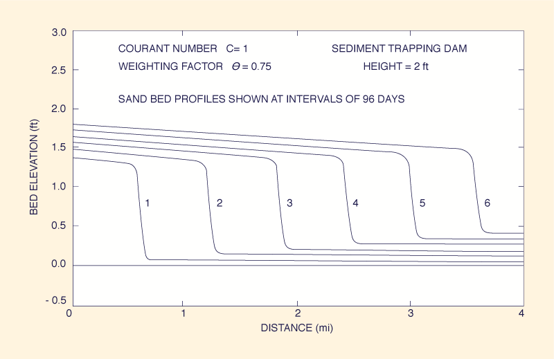
Erosional and Depositional Transients. The mathematical model may be used to study various erosional and depositional transients. The case of a sediment trapping dam is shown in Fig. 2.
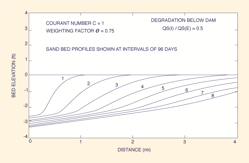
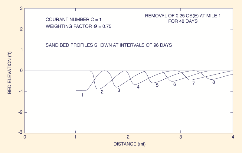
Other examples of transient formation and propagation such as the process of degradation below dams (Fig. 3) and the behavior of dredge cuts and borrow holes (Fig. 4) can similarly be studied using the mathematical model.
Modeling Variable Water Discharge. When modeling a time-varying water discharge inflow at the upstream boundary, the hydrograph is discretized into a number of intervals. Each interval is made to correspond to one or more bed transient time steps. The simulation of the time-varying water discharge is accomplished by interfacing a backwater computation between bed transient time steps.
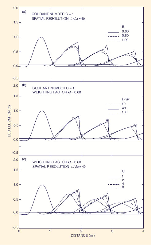
Sensitivity to Numerical Parameters. A series of test runs was designed with the purpose of assessing the sensitivity of the model to the numerical parameters. The problem is that of tracking the translation and attenuation of a sinusoidal sand wave as it travels downstream in a unit width channel. The physical parameters were set at Fo = 0.167, and σ* = 132. A sinusoidal sand wave of
Figures 5(a) to 5(c) show the results of the numerical testing. Fig. 5(a) shows that the larger the value of θ, the more stable the model, i.e., the larger the numerical dispersion introduced in the model. A value of θ = 0.6 shows a weak pattern of instability. Fig. 5(b) shows that low values of
Recommendations on Stability and Convergergence. Values of 0.5 ≤ θ ≤ 0.6 may result in a weakly stable or unstable solution. As a general rule, stability requires that θ > 0.6. A value of
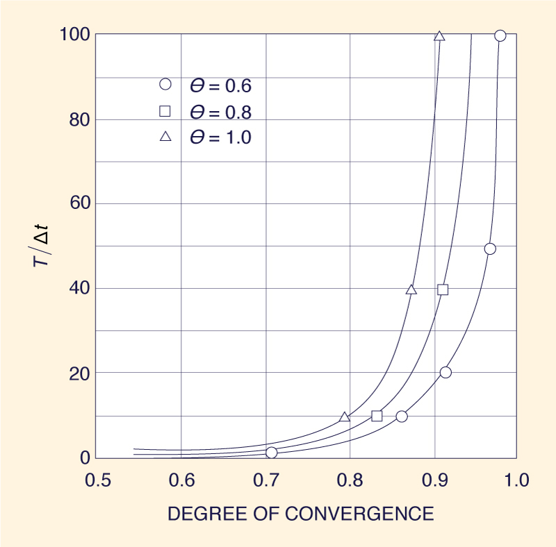
The second writer (7) has derived an approximate convergence criterion based on actual test runs. He defined a convergence parameter Cp as follows:
High values of Cp result in good convergence; conversely, low values of Cp are an indication of poor convergence. A lower limit of Cp may be dictated by accuracy considerations, while an upper limit may be necessary from the economic viewpoint. Eq. 16 can also be expressed as follows:
Figure 6 shows the results of the convergence analysis. The degree of convergence is defined as the ratio of numerical to analytical celerity, for numerical solutions with varying T/∆t and θ. Figure 6 underscores the importance of the temporal resolution T/∆t as the relevant convergence parameter while depicting the secondary role of the weighting factor θ. A recommended range for the temporal resolution is as follows: 20 ≤ T/∆t ≤ 100. Midrange values will represent a tradeoff between accuracy and cost constraints.
7. SUMMARY AND CONCLUSIONS A mathematical model is developed to simulate bed transient formation and propagation in alluvial channels. The model is of the known-discharge type, i.e., within one time step, the water discharge is considered steady. This technique allows for the implicit numerical modeling of bed transient propagation using longer time steps than would otherwise be possible using the conventional sequential routing method. Instability due to ill-posing of the sediment transport function is circumvented by using a power relation between bed material discharge and mean flow velocity. Errors in mass conservation due to a linearization at the boundary are eliminated by using a nonlinear formulation of the upstream boundary condition. The model can take account of time-varying water discharge by interfacing a backwater computation between one or a number of time steps. This feature allows for considerable flexibility in modeling long-term water surface and bed level transients.
Stability and convergence are analyzed, and criteria are established to ensure a successful model operation. In particular, convergence is shown to be primarily a function of the temporal resolution APPENDIX I. REFERENCES
APPENDIX II. NOTATION The following symbols are used in this paper:
C = bed transient Courant number, Chézy coefficient;
Cg = bed material transport coefficient;
Cp = convergence parameter, Eqs. 16 and 17;
Cs = spatial bed material concentration;
d = flow depth;
do = equilibrium flow depth;
Fo = Fronde number of equilibrium flow;
ƒ = a dependent variable;
ƒr = friction factor;
f = Darcy-Weisbach friction factor;
g = acceleration of gravity;
j = space discretization index;
L = characteristic length of transient;
L / ∆x = spatial resolution;
m = exponent in bed material transport function;
n = time discretization index;
p = bed porosity;
q = steady water discharge;
qs = bed material discharge;
qsL = Lateral sediment inflow;
Sf = friction slope;
So = bed slope;
T = characteristic duration of transient;
T / ∆t = temporal resolution;
t = time variable;
u = mean velocity;
x = space variable;
z = bed elevation referred to arbitrary datum;
∆ d1Q = change in flow depth at upstream boundary due to nonequilibritun water inflow;
∆ d1S = change in flow depths at upstream due to nonequilibrium sediment inflow;
∆ d1T = total change in flow depth at upstream boundary;
∆ ƒ = change in variable ƒ ;
∆ t = time step;
∆ x = space step;
δ = a real number;
θ = weighting factor of implicit scheme;
ρs = density of sediment particles; and
σ* = dimensionless wave number of transient. |
| 221013 |
| Documents in Portable Document Format (PDF) require Adobe Acrobat Reader 5.0 or higher to view; download Adobe Acrobat Reader. |