1. INTRODUCTION There exists a class of open-channel flow problems which can be adequately described in the context of depth-averaged, two-dimensional mathematical models. Essentially, these models are capable of resolving flow currents in two horizontal directions with the fluid and flow properties assumed to be invariant along the vertical. Such simplified representations of a three-dimensional phenomena are justified where turbulent mixing, due to bottom roughness, effectively generates a uniform velocity distribution over the flow depth. Thermal effluents from cooling facilities, contaminant discharges from chemical processing plants, and sediment movement by local scouring are all evidence of a progressive industrialization which has the potential to tax the natural cleansing action of waterways to the point where serious environmental consequences may result. Knowledge of the effect of proposed modifications is vital to the safe development and utilization of waterways. In this study, a fundamental investigation of the circulation phenomena in open channels is performed using a depth-averaged mathematical model. Circulation has been observed to have a primary influence on erosion and accretion processes, heat diffusion, and contaminant dispersion. Therefore, the clarification of the physical mechanisms leading to the generation of circulation in free-surface flow is a much needed research endeavor.
2. LITERATURE REVIEW
Prior to the development or efficient, high-speed computer
hardware, two alternatives were available to the researcher
interested in modeling free-surface flow: (1) analytical
solutions; and The increased efficiency of digital computers has triggered a continued research effort in the refinement of mathematical models. While offering almost unlimited flexibility in the simulation of alternatives, these models have the additional appeal of smaller development and operating costs. Certain specialized problems still remain within the realm of physical modeling, but the use of mathematical models continues to grow. Mathematical models of open channel flow exist at various levels of sophistication. The detailed description of flow phenomena is best accomplished in a three-dimensional spatial framework; however, the complexity of a formulation in three dimensions often requires large amounts of computational effort. Where valid, the simplification to a two-dimensional representation may offer a considerable reduction in complexity and expense. This involves an integration of the three-dimensional equations of fluid dynamics over the flow depth. The two-dimensional depth-integrated system of equations is not without its pitfalls: there is a closure problem associated with the effective shear stresses which act tangentially on vertical sides of a fluid element. No rigorous relation between these stresses and the depth-averaged variables is currently available. Hansen (6) is credited for being the first to outline the depth-averaged two-dimensional formulation. Later, several other researchers, notably Leendertse (10, 11), followed Hansen in applying Iwo-dimensional modeling concepts to the study of estuarine and coastal hydrodynamics. In a detailed analysis of free-surface flow, Leendertse developed a computational model for long-period wave propagation in well-mixed estuaries and coastal seas (10). Particular emphasis was given in Leendertse's work to the numerical properties of the two-dimensional model in the form of a linear stability and convergence analysis following the von Neumann approach.
Kuipers and Vreugdenhil (7) extended Leendertse's 1967 model
to the realm of secondary flows. In a companion report to that of Kuipers and Vreugdenhil, Flokstra (3) has directed attention to the importance of correctly modeling the effective shear stresses. Without actually resolving the closure problem associated with the modeling of these stresses, Flokstra made a detailed analysis of the relevant physical mechanisms contributing to the generation of circulation. According to Flokstra's vorticity balance, it is theoretically impossible to generate circulating flow without modeling the effective shear stress. In addition, Flokstra's analysis leads to the conclusion that a no-slip velocity condition at closed boundaries is essential to the generation of eddy flow patterns. Abbott and Rasmussen (1) verified Kuipers and Vreugdenhil's conclusion that the convective inertia terms are necessary for the generation of circulation. Using physical reasoning, they attributed the circulating patterns to a direct consequence of the resistance effects dominating the inertial effects. Abbott and Rasmussen also concluded that "pseudo-circulations," occurring strictly due to the truncation errors of first-order difference schemes, were possible in depth-averaged two-dimensional models. The occurrence of nonlinear instability in two-dimensional numerical models was also studied by Flokstra (4). Three approaches were cited to handle this problem: (1) A spatial smoothing process similar to that used by Kuipers and Vreugdenhil; (2) the explicit introduction of an eddy viscosity term in the equations of motion; and (3) the use of a difference scheme affected with numerical viscosity. McGuirk and Rodi (12) developed a depth-averaged velocity and contaminant distribution model of open-channel flow which described the recirculation region immediately downstream of a side discharge into a flowing river. Considering the constant turbulent diffusion coefficient and nonexplicit representations of the turbulent structure too crude for the side jet phenomena, McGuirk and Rodi utilized an extension of Launder and Spalding's (8) two-dimensional turbulence model. Lean and Weare (9) tested Flokstra's theoretically based conclusions using a-depth-averaged circulation model of flows past a breakwater. The effective stresses were shown to have contributions from shear layer turbulence and turbulence generated at the bed. Criteria is presented to delimit the conditions under which the shear layer turbulence will predominate. An observation of numerical circulation (5) similar to that experienced by Abbott and Rasmussen but caused by a coarse computational grid is reported. At present, many uncertainties exist in the mathematical modeling of depth-averaged two-dimensional open-channel flow. Several models which exhibit circulation and numerous theoretical reviews on the factors causing circulation are present in the literature. However, no comprehensive analysis of the various mechanisms leading to circulation has been attempted in conjunction with a numerical model. The objectives of this study are, thus, twofold: (1) the clarification of the physical processes which contribute to the generation of circulation; and (2) the identification of significant factors in the numerical specification of circulating flow problems. 3. GOVERNING EQUATIONS The derivation of the equations governing depth-averaged free-surface flow is accomplished by the successive simplification of the general three-dimensional fluid flow equations. i.e., the Navier-Stokes equations. Four assumptions are basic to the equation set used in this study: (1) water is incompressible; (2) vertical velocities and accelerations are negligible; (3) wind stresses and geostrophic effects are negligible; and (4) average values are sufficient to describe properties which vary over the flow depth. Fluid density effects are not considered in this study; thus, incompressibility is a limitation to the applicability of the model. The second assumption is a consequence of the relatively large magnitude of the gravitational body force which, in flows of shallow depth, simplifies the z-component of the motion equation to a statement of hydrostatic pressure distribution in the vertical. For the type of flow under consideration, i.e., open-channel flow, the magnitude of the wind and geostrophic effects is insignificant compared to the driving forces found in the mean flow currents. These two terms can be easily incorporated into the model if desired, and their absence does not detract from the generality of the conclusions of this study. The most significant assumption is that an average value is capable of representing a property which normally varies over the flow depth. Until this assumption is made, the analysis is fundamentally three-dimensional. Due to the depth-averaging of the equation set, information on the vertical distribution of velocity is partially lost. Fortunately, the shallow waters found in rivers and well-mixed estuaries usually do not require such detailed information. The resulting depth-averaged equations are:
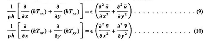
in which ū, v̄ = depth-averaged velocities; t = time; x, y = coordinate directions; g = gravitational acceleration; η = water elevation (η = h + zb); ρ = fluid density; τbx, τby = bottom shear stresses; and Txx, Txy, and Tyy = effective shear stresses defined as follows:
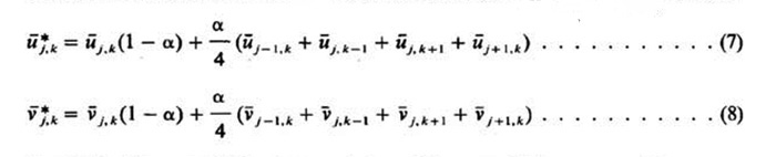
in which ν = kinematic viscosity; and u' and v' = turbulent velocity fluctuations. The foregoing equation set, although containing many approximations and simplifications, is not closed. Historically, turbulent flow theory has suffered from an incomplete physical representation of the turbulent momentum transfer (Reynolds stresses), i.e., those stresses due to the correlations of turbulent velocity fluctuations. Depth-averaging the formulation further complicates the problem by creating an additional stress due to the nonuniform velocity distribution in the vertical. These two stresses and the viscous shear stress combine into the terms previously identified as the effective shear stress. Representing the effective shear stresses in terms of the mean flow variables is by far the largest impediment to the proper depth-averaged modeling of circulating flow. Since this problem remains to be solved, the use of empirical parameters and calibration techniques is indicated. In this study, the procedure developed by Kuipers and Vreugdenhil (7) is adopted. This particular technique does not explicitly include the effective shear stresses in the equation set, but introduces them in a velocity-averaging routine which effectively simulates the contribution of the effective stresses. In this routine, an averaging procedure occurs after each set of new dependent variables has been generated, as follows:
in which ūj,k* = spatially averaged ūj,k; v̄j,k* = spatially averaged v̄j,k; α = weighting factor; and j,k = spatial indices. When these substitutions are made in the governing equations, closure terms appear such that
in which ∈ = α (Δx)2 /(2Δt ); Δx = spatial increment; and Δt = temporal increment.
The bottom shear stress,
like the effective shear stress, has not been rigorously
related to flow properties. However, years of experimentation
has resulted in the development of several
empirical resistance equations. Any of the applicable
resistance equations may be used to relate the bottom
shear stress to the flow velocity, assuming the validity
of a steady uniform flow roughness.
in which fr = g /C 2 and C = Chezy coefficient. 4. MATHEMATICAL MODEL
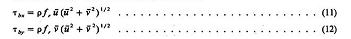
A finite difference approximation is used to represent the partial differential equation set in the numerical model. In order to visualize the computational structure, the reader must imagine levels of horizontal x-y grids layered in the vertical time dimension. Conceptually, the four variables, u, v, η, and zb should all be defined at every node location. However, practical limitations in the computational procedure make it more convenient to define a separate grid system for each of these variables. These four grid systems are staggered in space in a form originally due to Platzman (13), as shown in Fig. 1. Normally, it is not necessary for Δx to be equal to Δy; however, the representation of the effective shear stresses used in this model does hinge on this assumption.
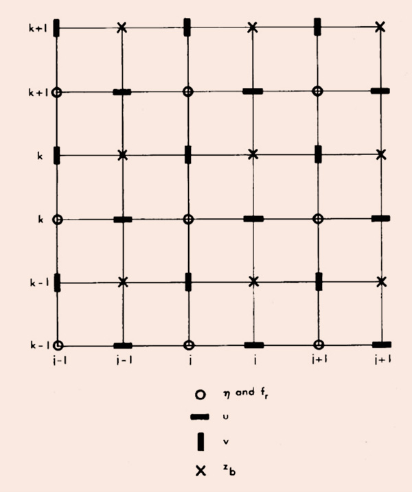
Among the several types of finite difference schemes available, the central difference approximations provide second-order accuracy. Generally speaking, spatial derivatives can always be expressed in a central difference format. However, unless iterations are performed, temporal derivatives cannot be represented by central difference schemes because two entire time levels of unknowns would be present. The additional computational effort required by an iterative formulation is normally not warranted. Consequently, a less accurate but more expedient first-order difference scheme is preferred for the temporal derivatives. Equations which are nonlinear with respect to the unknown variables present formidable difficulties for an efficient numerical solution. Although the governing equations contain nonlinear terms, a judicious specification of known and unknown values in the finite difference equations results in a linear representation of the unknown variables. This equation set is then solved by an efficient matrix inversion algorithm. The computational procedure used in this model is a multioperational solution mode based on the division of each time step Δt into two stages of half-time step each. Leendertse (10) modified the well-known "alternating-direction implicit" or ADI method, by including two explicit schemes in such a way that each stage contained an implicit scheme followed by an explicit scheme. The advantage of the ADI method, in addition to those attributable to implicit schemes, lies in the solution procedure which solves the x-momentum equation separately from the y-momentum equation, permitting the two-dimensional problem to be solved as a sequence of two one-dimensional problems. After each implicit step, a single dependent variable remains unknown and can be directly solved for by an explicit method. The numerical model is based on the set of governing equations derived earlier. Each of the three equations has a difference scheme centered about a unique location on the grid system. The x-momentum equation is referenced to the node occupied by ūj,k while the y-momentum equation is centered about node location v̄j,k; ηj,k is the reference location for the continuity equation (for simplicity, overbars are omitted hereafter). In the mathematical model used in this study. the finite difference analogs of the various equations are, for the first stage:
Similar discretization techniques are applicable for the second stage: (1) y-momentum and continuity (implicit): and (2) x-momentum (explicit). See Ref. 14 for additional details.
Two boundary types may be
specified in the numerical model: closed and open
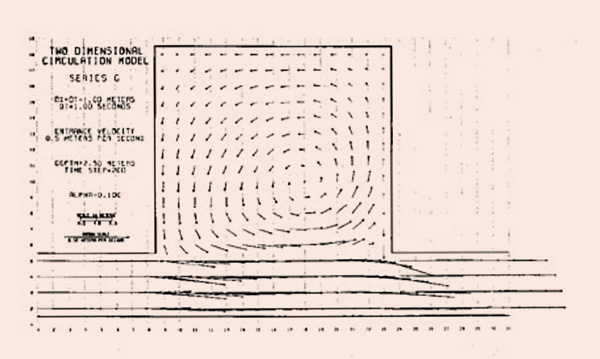
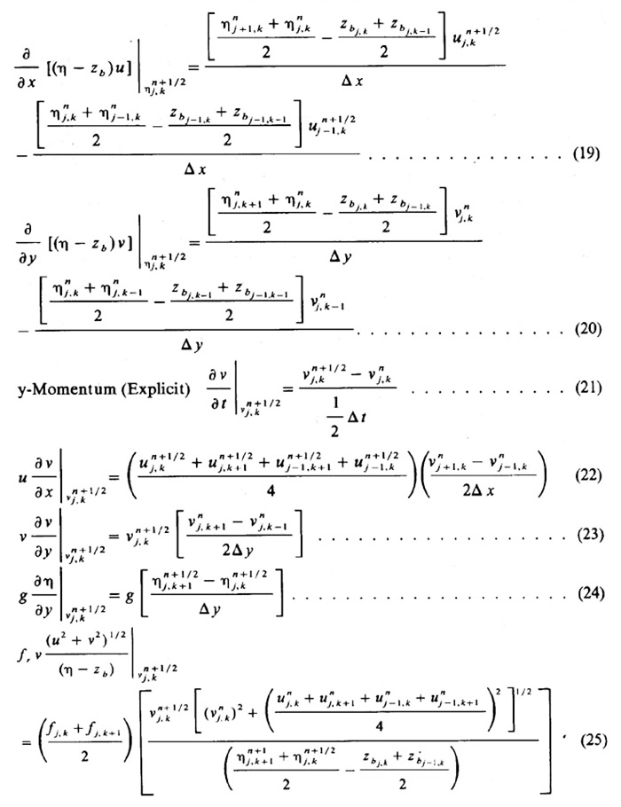
boundaries. Spatial central finite differences such as those used in this model require information which lies outside the boundaries of the computational model. Although a zero velocity tangential to the wall is a realistic assumption (the no-slip velocity condition), a zero water level at the boundary can be grossly inaccurate and may lead to numerical stability problems. A satisfactory alternative appears to be the relocation of interior values. A simple relocation technique was chosen, in which exterior values were defined to be equal to those interior values adjacent to the boundaries. This is tantamount to a perfect slip condition, a reasonable assumption in turbulent flows in which the viscous effects have little influence on the horizontal velocity distribution. A pervasive problem in two-dimensional mathematical modeling is the lack of adequate theoretical numerical stability criteria. Linear stability theory classifies the multi-operational procedure as unconditionally stable. However, experience (15) has shown that it is only weakly stable. 5. RESULTS The objective of the numerical experimentation is the clarification of the circulation phenomena found in free-surface flow. Two hypothetical configurations are tested under various initial and boundary conditions. In addition to a sensitivity analysis, experiments are performed in which more than one element is varied from the baseline in order to determine the interaction between several components. The bulk of the testing program consists of experiments performed on a channel-pool configuration. Channel dimensions are 4 m in width by 30 m in length, while the pool is a rectangle 14 m wide and 15 m long. The first series of tests are performed with a 0.5 m/s velocity specified in the channel as an initial condition and at the upstream end as a steady boundary condition. A water depth of 2.5 m serves as both the initial condition and the steady downstream boundary condition. There is no velocity in the pool initially. Closed boundaries are represented by zero velocities perpendicular to walls. Without a bed slope, the water in the system is driven solely by the upstream entrance velocity. Numerical parameters used in the baseline run are weighting factor α = 0.1, friction factor fr = 0.0045, spatial increment Δx = Δy = 1 m, and temporal increment Δt = 1 sec. Figure 2 is a plot of the baseline velocity vectors after 200 sec of simulation. A well-developed circulation appears in the pool area with little or no divergence from the mainstream flow. Water levels in the pool range from 2.50 m to 2.52 m. Entrance levels. however, fall continuously from 2.50 m to 2.44 m.
The necessity of modeling the effective shear stresses where physical circulation is present has been explained theoretically by Flokstra (3). In the present model, the representation of the effective shear stresses is not explicit in the discretized equation set; rather, the action of the effective shear stresses is simulated by a velocity-averaging interphase which employs a weighting factor α to control the magnitude of the effect. The first experiment performed on the channel-pool configuration omits the effective stress modeling by setting α = 0. Transfer of turbulent momentum from the mainstream to the pool is insignificant in this case. With no flow divergence into the pool, the initial conditions are virtually preserved.
The convective inertia terms, u ∂u/∂x,
v ∂u/∂y,
u ∂v/∂x, and
v ∂v/∂y,
are often neglected in numerical modeling because the nonlinearity of
these terms introduces additional complexities.
In the literature, the role of friction
in circulation is not clearly defined. To shed more light on fhis subject,
an experiment is performed wherein the friction terms,
The effect of an increase in flow depth
has been documented by Bengtsson (2) following experiments performed on a lake model.
His conclusion was that the influence of the horizontal turbulence terms was reduced with increasing depth.
In this study, the horizontal dispersion of momentum is simulated by the effective stress closure terms,
The earlier experiments
with friction appear to dismiss the importance attached to it by some authors. However, these tests were
all performed on problems of relatively small scale. To test the effect of friction in a large-scale problem,
the size of the configuration was increased by setting
In earlier tests, a perfect-slip velocity condition
had been implemented at all closed boundaries with satisfactory results. To test the validity of this
assumption, an experiment is performed in which the flow is subject to a no-slip velocity condition as
closed physical boundaries. This condition can be approximated by setting all velocities located
outside of the physical boundaries to zero. For this experiment, a bed slope So = 0.0005 is introduced
into the channel-pool configuration. Secondary flow in sudden expansions is of a slightly different nature than the channel-pool system treated earlier. This is due in part to the bending of currents into the expansion and the increased exposure of secondary currents to mainstream effects. Abbott and Rasmussen (1) developed a channel expansion model from which results and conclusions were presented. An attempt is made here to verify these conclusions using a similar geometry.
In this testing series, the configuration consists of an entrance channel 9 m wide and 7.5 m long while
the expanded channel is 17 m wide and 22.5 m long. A fixed bed slope of So = 0.0005 in the direction of
the entrance channel flow in specified for the entire configuration. The initial condition is a water surface
slope parallel to the bed at a depth of 2.5 m. All velocities are set to zero at the beginning of the simulation.
Open boundary conditions at both upstream and downstream ends are water levels which match the initial
conditions. Closed boundaries are zero velocities
perpendicular to the walls. Friction in this model
is governed by a dimensionless friction factor fr = 0.0045.
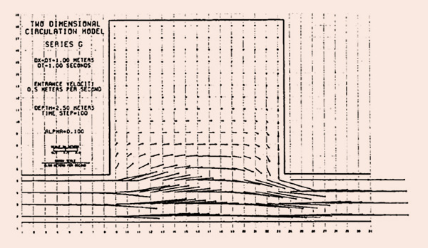
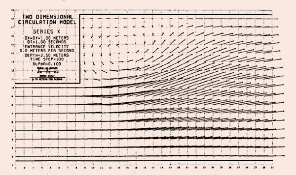
For the most part, the testing of the channel expansion produced results consistent with those of the channel-pool configuration. A discrepancy was found, however, when the slope-specified models were tested without modeling the effective stress. In the velocity-specified channel-pool model, the absence of the effective stresses resulted in no circulation being produced. Contrary to this result, both configurations, i.e., the channel expansion and the channel-pool system, are able to generate a spiraling secondary flow without the presence of the effective stresses if a bed slope is the driving force. The question arose that the secondary currents which appear without the benefit of effective stress modeling may be of a strictly numerical nature. Theoretically, numerical effects should be minimized as the discretization domain is made exceedingly small. To this end, both space and time increments in the expansion model were reduced although the problem size remained constant. The values of these parameters for this test are Δx = Δy = 0.5 m and Δt = 0.5 sec. A horizontal water surface without velocity is specified as the initial condition. As the simulation begins, the downstream water level is lowered in 40 time steps to a depth of 2.5 m, the same depth as the upstream boundary condition. Thus, a line drawn through the end point water levels will be parallel to the bed slope. The weighting factor for this experiment is zero while the nondimensional friction factor is 0.0095. Figure 5 is a plot of the velocity vectors after 150 sec of simulation. A strong spiraling "circulation," with a character similar to those observed in earlier slope-specified experiments, sets up in the expansion corner.
6. EVALUATION The testing program for this study is fairly extensive; therefore, only a limited discussion can be presented here. However, the analysis and evaluation of the numerical experiments is based on all the tests performed. For a more detailed description, the reader in referred to Ref. l4. The use of specified water levels at the open boundaries proved to be a better boundary condition than the velocity specified in the early testing series. When a difference in water levels is the driving force for flow through the configuration, both velocity and water surface are steady and continuous, with few, if any, anomalies. This is in contrast to the velocity-specified model which requires a special initial condition before simulation can begin. In addition, oscillating water levels and velocities plague any of the velocity-specified simulations.
Specific differences in model behavior due
to a change in boundary conditions are found only in the testing of α, the
weighting factor used in the velocity-averaging routine. In the velocity-specified
model, circulation did not occur without the presence of the closure
terms,
While acknowledging the "no-slip" velocity condition in nature, the testing of this model has been performed primarily with a "perfect slip" boundary specification. This is a reasonable assumption in models where the spatial resolution across a channel width is not very fine. In the experiment involving the specification of zero velocities outside the boundary geometry, overwhelming resistance effects resulted. Obviously, any consideration of a no-slip boundary condition must be coordinated with an accompanying reduction in the bed resistance effects.
Results from the
testing program are reasonable and encouraging, despite the presence of two flaws traceable
to the representation of the effective stresses. First, there is yet to be found a physical
basis by which to choose the appropriate weighting factor, α, of the velocity averaging routine.
The second drawback in the effective stress representation is somewhat more serious than the first. Much of the success is fulfilling the required profile of traits by the closure terms is due to the effect of numerical viscosity. As the weighting factor is increased, the model reacts as if the fluid is becoming more viscous, thus increasing the exchange of lateral momentum and increasing viscous damping. Essentially, viscosity is used to model a turbulence effect. Therefore, care must be exercised when using the velocity averaging routine. A balance must be struck between the simulation of the effective stresses and the associated change in fluid properties. This study has experimentally verified Flokstra's conclusion that true circulation, i.e., a flow pattern possessing a separation zone with closed circular streamlines, requires the modeling of the effective shear stresses. An order-of-magnitude analysis performed on the various terms in the equation of motion confirms the significance of the effective stresses in all instances where circulation occurs. Circulation requires a continuous exchange of turbulent energy across the shear layer to be maintained. Withdrawal of the effective stresses after the steady flow pattern has set up dissolves the circulation and ultimately leads to instability.
The
order-of-magnitude analysis of terms found in the momentum equation shows that convective inertia
is significant in the channel and shear layer for all instances where circulation occurs. Merely including the convective inertia in the mathematical model will not ensure the generation of secondary flow. Even with the additional stipulation that the effective stresses and all other quantities be precisely described, circulation may yet be inhibited by frictional effects. In every case where secondary currents do not occur, the resistance term is significant and larger than the convective inertia terms.
This study has found that bottom friction is the largest deterrent to
the existence of circulating flow.
This model displays at least
two different instability mechanisms: Nonlinear and Courant. Nonlinear instability is characterized by gradually developing water surface discontinuities accompanied by a similar behavior in the computed velocities. The process is usually slow, and can take as many as 100 time steps to develop. In this numerical model, nonlinear instability requires that the velocity averaging technique be present in all simulations although the weighting factor need not be large. Most runs were stable with α = 0.1. Physically speaking, the use of the velocity-averaging routine introduces a stronger viscous dissipation mechanism into the fluid. Energy no longer must be transferred to scales smaller than the grid resolution for viscous effects to act. Courant instability occurs when the ratio of physical celerity to numerical celerity (defined as the Courant number) exceeds a characteristic value. The physical celerity for this model is the maximum channel velocity, Umax, while the numerical celerity is defined as Δx/Δt = Δy/Δt. Thus, the criterion is of the form Umax (Δt /Δx) ≤ ε, in which ε is the characteristic limit. The two explicit stages contained in the multioperational procedure are presumably responsible for the Courant stability condition found in this model. Courant instability is characteristically a very rapid process. The simulation proceeds without noticeable difficulty until a sudden discontinuity appears in one of the dependent variables. Within a few time steps the entire calculation is spoiled. In this study the limiting value of the Courant number is dependent upon the weighting factor used in the velocity averaging routine. This is to be expected since large weighting factors can smooth instabilities that would otherwise occur if smaller weighting factors were used. For α = 0.1, the Courant number in this model must be less than or equal to 0.5. 7. CONCLUSIONS AND RECOMMENDATIONS Major conclusions from this study are as follows:
The following recommendations are offered for future research:
ACKNOWLEDGEMENTS
This study was made possible by a National Science Foundation
Grant No. CME-7805458.
APPENDIX I. REFERENCES
APPENDIX II. NOTATION The following symbols are used in this paper:
|
| 211227 |
| Documents in Portable Document Format (PDF) require Adobe Acrobat Reader 5.0 or higher to view; download Adobe Acrobat Reader. |