1.  INTRODUCTION

The Muskingum-Cunge flood routing model is well established in hydrologic engineering practice. The model can simulate the convection and diffusion of flood waves in an expedient and accurate manner (Cunge 1969; Ponce and Yevjevich 1978; Ponce et al. 1996). The convection is characterized by the wave celerity, defined as the slope of the discharge-area rating divided by the top width (Seddon 1990; Chow 1959). The diffusion is characterized by the hydraulic diffusivity, defined as one-half of the unit-width discharge divided by the water surface slope (Hayami 1951).

The conventional Muskingum-Cunge model is based on kinematic wave theory; thus, it uses the equilibrium or bottom slope in the expression for hydraulic diffusivity. This assumption leads to a single-valued rating, which limits the model in certain cases. In this paper, we extend the Muskingum-Cunge model to the realm of looped dynamic ratings. This is accomplished by reformulating the Muskingum-Cunge algorithm to use the local water surface slope and the Vedernikov number in the expression for hydraulic diffusivity. This makes possible the simulation of looped ratings, which more closely resemble the actual flood wave propagation. To assess the accuracy of the computation, we compare our looped ratings with those calculated using a dynamic wave model (Liggett 1975; Liggett and Cunge 1975; Fread 1993).

2.  MUSKINGUM-CUNGE ROUTING MODEL

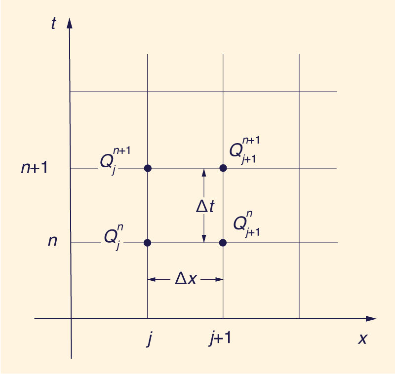
The conventional Muskingum-Cunge model is well established (Cunge 1969; Ponce and Yevjevich 1978; Ponce 1986; HEC-1 1990). The routing equation, including lateral inflow/outflow, is the following (Fig. 1):

Fig. 1  Schematic of x-t plane for Muskingum-cunge model.

Q j+1 n+1 = CoQ j n+1 + C1Q j n + C2Q j+1 n + C3QL

(1)

in which j = spatial index; n = temporal index; and Q_L = lateral flow (source or sink). The routing coefficients are the following:

-1 + C + D            Co  =  ____________             1 + C + D

(2)

1 + C - D            C1  =  ____________             1 + C + D

(3)

1 - C + D            C2  =  ____________             1 + C + D

(4)

2C            C3  =  ____________             1 + C + D

(5)

in which C and D = Courant and cell Reynolds numbers, respectively.

The Courant number is the ratio of the flood wave celerity c to the grid celerity ∆x /∆t, such that:

∆t            C  = c  _____              ∆x

(6)

The cell Reynolds number is the ratio of the hydraulic diffusivity q / ( 2S ) (Hayami 1951) to the grid diffusivity (c∆x / 2) (Ponce and Yevjevich 1978), such that:

q            D  =  _________            S c ∆x

(7)

in which q = unit-width discharge; and S = channel slope.

In the conventional Muskingum-Cunge model, channel slope is approximated by bottom slope (in prismatic channels) or equilibrium slope (in natural channels). In the linear mode of computation, the routing parameters are based on reference flow values and are kept constant throughout the computation in time. This mode of computation is referred to as the constant-parameter method (Dooge 1973), to distinguish it from the variable-parameter method, in which the routing parameters are allowed to vary with the flow (Ponce and Yevjevich 1978).

In the nonlinear mode, the routing parameters are based on average values of q and c at each computational cell. This can be achieved with a direct three-point average of the values at the known grid points, or by a iterative four-point average, which includes the unknown grid point (j + 1, n + 1) (Ponce and Chaganti 1994). To improve convergence, the three-point average is used as the first guess at the iteration. Channel slope S remains unchanged within each computational cell.

A recent extension of the Muskingum-Cunge model enables it to partially account for the flow dynamics. This is accomplished by modifying the hydraulic diffusivity to include the Vedernikov number (Dooge et al. 1982; Ponce 1991), effectively converting it into a dynamic hydraulic diffusivity ν_d :

q            νd  =  ____ ( 1 - V 2 )            2S

(8)

in which V = Vedernikov number, defined as the ratio of relative kinematic wave celrity to relative dynamic wave celerity (Vedernikov 1945, 1946; Craya 1952). Thus, when the Vedernikov number is equal to 1, the hydraulic diffusivity vanishes. With Eq. 8, the cell Reynolds number is now defined as follows:

q            D  =  _________ ( 1 - V 2 )            S c ∆x

(9)

3.  LOOPED-RATING MUSKINGUM-CUNGE MODEL

According to flood wave propagation theory, wave diffusion invariably produces a looped rating; i.e., for a given stage, the discharge is higher in the rising limb than in the receding limb. The loop thickness increases as the wave becomes more diffusive, and coalesces to zero as the wave becomes more kinematic.

In the cases where the loop exists and is significant, its calculation may portray more accurately the nature of flood wave propagation. In Muskingum-Cunge routing, the looped rating can be accounted for by using the local water surface slope in the expression for hydraulic diffusivity.

A looped-rating Muskingum-Cunge model was developed by modifying the four-point variable-parameter model (Ponce and Chaganti 1994). Unlike the conventional model, the looped-rating model uses flow depths as an intrinsic part of the computation. For each computational cell, the procedure consists of the following steps:

1. Flow depth at point ( j + 1, n + 1 ) is used, together with the other three known flow depths in the cell to calculate the average cell water surface slope and flow depth. To improve the convergence of the iterative procedure, the result of the conventional four-point calculation is used as a first guess of the iteration.

2. The cell water-surface slope and flow depth are used, together with the Manning equation, to develop a rating, from which a reference discharge and celerity are calculated.

3. The cell flow depth, reference discharge, and celerity are used to calculate the routing parameters (Eqs. 6 and 9), from which the routing coefficients are calculated (Eqs. 2 to 5).

4. Using Eq. 1 and the routing coefficients, a new discharge at point (j + 1, n + 1) is calculated.

5. The new discharge and the rating developed in step 2 are used to calculate a new flow depth at (j + 1, n + 1).

6. The procedure is repeated (steps 1 to 5) until the difference between two consecutively calculated discharges (in step 4) is within a small, specified tolerance.

4.  NUMERICAL EXPERIMENTS

A program of numerical experiments was devised to test the looped-rating Muskingum-Cunge algorithm. A hydraulically wide channel was assumed so that computations could be carried out in terms of unit-width discharge and flow depth. This ensures that the routing remains one-dimensional, thereby avoiding the complexities associated with channel overflows.

The bottom slope was fixed at S_o = 0.0005 and a channel length L = 200 km was chosen. For this bottom slope and channel length, the amount of wave diffusion is sufficient to produce a measurable loop at the downstream end.

A Manning friction coefficient n = 0.04 was selected. Since the channel is hydraulically wide, the exponent of the rating is β = 5/3 (Chow 1959). The following two baseflow values were chosen: q_b = 1 and 2 m² s^-1. The following two peak-inflow/baseflow ratios were chosen: q_pi / q_b = 2 and 5.

The inflow hydrograph was assumed to be

qpi + qb     qpi - qb          2π t qi  =  ________ - ________ cos _____                2              2                T

(10)

where q_i = inflow at time t; q_pi = peak inflow; and T = flood wave period (Thomas 1934; Dooge 1973). The following three wave periods were chosen: T = 24, 48, and 96 h. These wave periods are within the diffusive wave range for these flow conditions (Ponce et al. 1978b).

Two resolution levels were chosen, resolution Ι with ∆x = 10 km, and ∆t = 3 h; and resolution ΙΙ with ∆x = 5 km, and ∆t = 1.5 h. With resolution Ι, the number of space steps is 20; with resolution ΙΙ, the number of space steps is 40. The total simulation time was set at five times the wave period. The total number of time steps is a function of resolution level (Ι or ΙΙ) and wave period (24, 48, or 96 h). For example, for resolution Ι and T = 96 h, the number of time steps is 5 × (96 / 3) = 160.

The testing program varied the following four parameters, for a total of 24 runs:

1. Resolution level (Ι and ΙΙ)

2. Flood wave period (24, 48, and 96 h)

3. Baseflow (1 and 2 m² s^-1)

4. Peak-inflow / baseflow ratio (2 and 5).

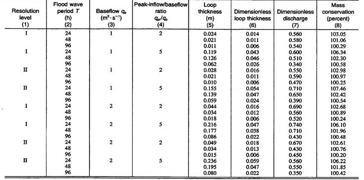
A summary of the results is shown in Table 1. All 24 runs showed a measurable loop in the discharge-depth rating. Loop thickness is taken as the maximum difference between the flow depths of the rising and receding limbs.

Dimensionless loop thickness is defined as the loop thickness divided by the average of the two flow depths (measured at the loop thickness). Dimensionless discharge (at the loop thickness) is defined as the difference between discharge (at the loop thickness) and baseflow, divided by the difference between peak outflow and baseflow. Mass conservation (in percentage) is defined as the ratio between the outflow and inflow hydrograph volume, excluding baseflow, multiplied by 100.

Table 1 shows that as the period increases (column 2), the wave becomes more kinematic and the loop thickness decreases (columns 5 and 6). Conversely, as the period decreases, the wave becomes more diffusive and the loop thickness increases. These results are in agreement with established flood wave propagation theory (Lighthill and Whitham 1955).

The loop thickness (column 5) varied between 0.010 and 0.236 m, and the dimensionless loop thickness (column 6) varied between 0.006 and 0.059 (0.6% and 5.9%, repectively). Both loop thickness and dimensionless loop thickness increase as the flow becomes more diffusive. The dimensionless discharge (column 7) varies between 0.35 and 0.74, with the lower values being associated with the longer periods, for which the flow is more kinematic.

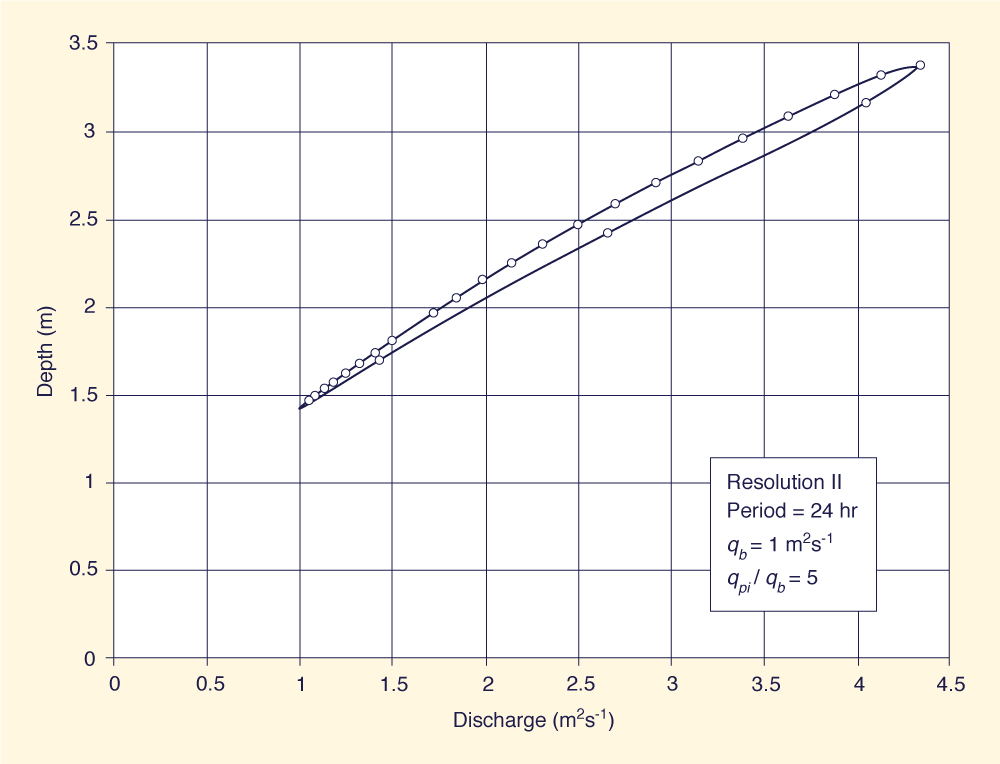
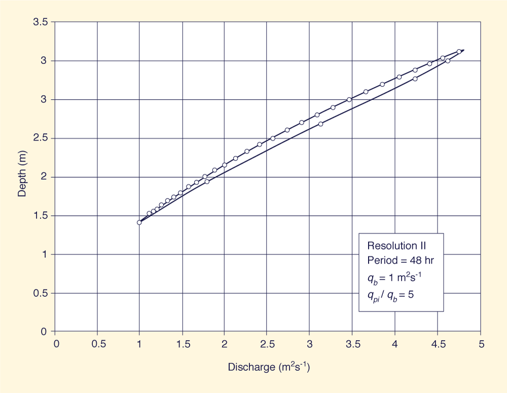
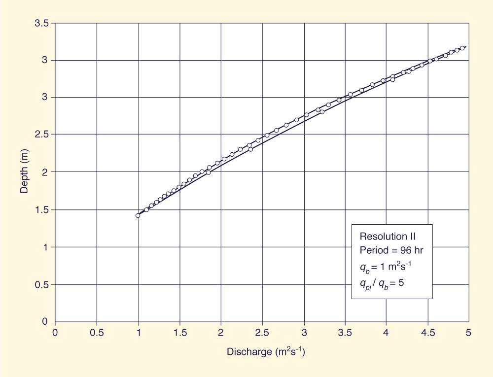
Table 1 shows that the looped-rating Muskingum-Cunge algorithm has a slight tendency to artificially gain mass (column 8). The mass gain increases with loop thickness and peak-inflow / baseflow rario. Attempts to develop a Muskingum-Cunge algorithm that produced a loop rating while conserving mass exactly were not successful. The relatively small mass gain is judged to be within the normal accuracy of hydrologic engineering computations. Figs. 2(a)-2(c) show typical looped ratings generated by the Muskingum-Cunge model, corresponding to resolution ΙΙ; wave periods of 24, 48, and 96 h; baseflow = 1 m² s^-1; and peak-inflow/baseflow ratio = 5.

Table 1.  Summary of results using the looped-rating Muskingum-cunge model.

Fig. 2 (a)  Typical looped ratings generated by the Muskingum-cunge model; period = 24 h.

Fig. 2 (b)  Typical looped ratings generated by the Muskingum-cunge model; period = 48 h.

Fig. 2 (c)  Typical looped ratings generated by the Muskingum-cunge model; period = 96 h.

5.  COMPARISON WITH DYNAMIC WAVE MODEL

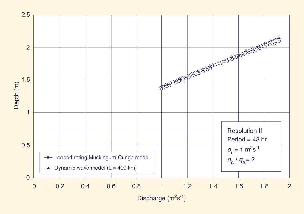
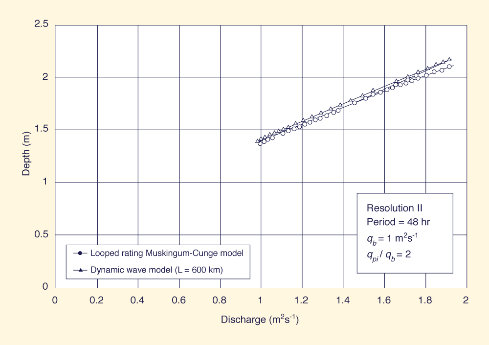
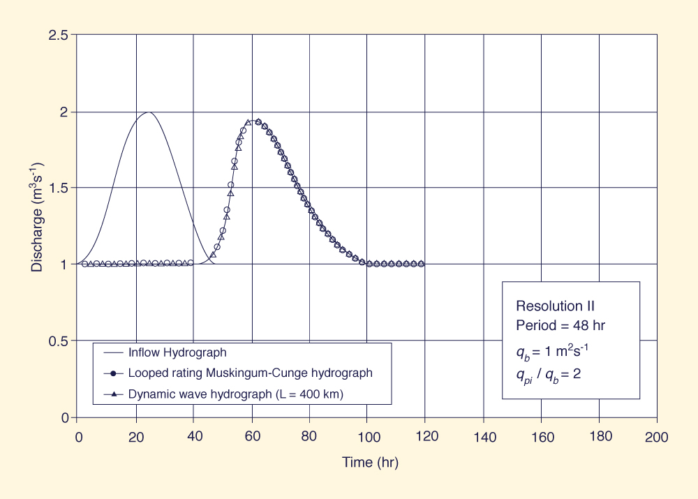
The looped ratings generated by the Muskingum-Cunge model were compared with ratings generated using DYNA, a dynamic wave model based on the St. Venant equations (Ponce 1982). A significant feature of a dynamic wave model is that it requires the specification of a downstream boundary condition. Since the looped rating is not known beforehand, a single-valued rating is usually assumed. However, the single-valued rating contradicts the solution at the boundary and affects the calculated results upstream (Abbott 1976).

In practice, the looped rating at the downstream boundary can be modeled in one of two ways: (1) by using the friction slope in lieu of the bottom slope, in a procedure that closely resembles the looped-rating Muskingum-Cunge algorithm (Fread 1993); or (2) by artificially extending the channel to specify a single- valued rating at a section farther downstream, while giving the loop a chance to develop at the upstream cross section of interset. Sensitivity analyses using several lengths of channel extension can provide a guide to determine the appropriate length.

For the purpose of comparison, a subset of the original testing program (resolution ΙΙ; periods of 24, 48, and 96 h; a baseflow of 1 m² s^-1; and a peak-inflow / baseflow ratio of 2) was run with the dynamic wave model. Since the channel reach length for the testing program is 200 km, the model was run using 400 km and 600 km channel lengths.

A key parameter of the Preissmann scheme (featured in DYNA) is the weighting factor θ, which is used to control numerical instability. Theoretically, a value of θ = 0.5, although second-order accurate, is unable to control nonlinear instabilities that sometimes plague dynamic wave computations. Offsetting the scheme to the stable side, i.e., increasing the value of θ above 0.5, will increase stability at a cost of reduced convergence (O'Brien et al. 1951; Ponce et al. 1978a). In practice, values of θ between 0.5 and 0.6 are commonly used to achieve a workable compromise between stability and convergence (Fread 1993).

In dynamic wave routing, the choice of weighting factor is the responsibility of the modeler. In our case, several values of θ were tried in order to determine the most suitable value. The larger values of θ eliminated numerical instabilities, but at the cost of decreased convergence (a substantial reduction of peak flow). A value of θ = 0.55 was chosen to closely match the dynamic wave model results with those of the looped-rating Muskingum-Cunge model.

Figures 3(a) and 3(b) show typical looped ratings for the Muskingum-Cunge and dynamic wave models, at a distance of 200 km. In the case of the dynamic wave model, the looped rating was produced by the artificial extension of the channel. The looped ratings (at 200 km) for the 400 km and 600 km channel lengths shown in Figs. 3(a) and 3(b) were essentially the same. Therefore, it is concluded that the 400 km channel length was sufficient to produce an accurate looped rating at the cross section of interset (at 200 km). Fig. 4 shows outflow hydrographs for the looped-rating Muskingum-Cunge and dynamic wave models. Only the dynamic wave model results for L = 400 km are shown. There is substantial agreement between the outflow hydrographs calculated by both models.

Fig. 3 (a)  Typical looped ratings generated by the Muskingum-cunge and dynamic wave models at a distance of 200 km, with L = 400 km.

Fig. 3 (b)  Typical looped ratings generated by the Muskingum-cunge and dynamic wave models at a distance of 200 km, with L = 600 km.

Fig. 4  Comparison of outflow hydrographs generated by the looped rating Muskingum-cunge and dynamic wave models at a distance of 200 km.

6.  SUMMARY AND CONCLUSIONS

A looped-rating Muskingum-Cunge model was developed by reformulating the conventional four-point model to use the local water surface slope and the Vedernikov number in the expression for hydraulic diffusivity. The developed model was successful in generating looped ratings under a wide range of kinematic/diffusive unsteady flow conditions, i.e., within the range of applicability of the Muskingum-Cunge method (Ponce et al. 1978b; Ponce and Yevjevich 1978).

A program of numerical experiments was used to test the looped-rating Muskingum-Cunge model. Resolution level, flood wave period, baseflow, and peak-inflow/baseflow ratio were varied to determine loop thickness, dimensionless loop thickness, dimensionless discharge, and percentage mass conservation. Comparison of the looped-rating Muskingum-Cunge model with a more complex dynamic wave model (DYNA) showed that both models are capable of generating looped ratings and outflow hydrographs of comparable accuracy.

APPENDIX I.  REFERENCES

Abbott, M. A. 1976. "Computational hydraulics: A short pathology." J. Hydr. Res., Delft, The Netherlands, 14(4), 271-285.

Chow, V. T. 1959. Open-channel hydraulics, McGraw-Hill, New York.

Craya, A. 1952. "The criterion for the possibility of roll-wave formation." Gravity Waves: Circular No. 521, National Bureau of Standards, Washington, D.C., 141-151.

Cunge, J. A. 1969. "On the subject of a flood propagation computation method (Muskingum method)." J. Hydr. Res., Delft, The Neterlands, 7(2), 205-230.

Dooge, J. C. I. 1973. "Linear theory of hydrologic systems." USDA Tech, Bull. 1468, U.S. Department of Agriculture, Washington, D.C.

Dooge, J. C. I., W. B. Strupczewski, and J. J. Napiorkowski. 1982. "Hydrodynamic derivation of storage parameters of the Muskingum model." J. Hydro., Amsterdam, 54, 371-387.

Fread, D. 1993. "Chapter 10: Flow routing." Handbook of hydrology, D. R. Maidment, ed., McGraw-Hill, New York.

Hayami, S. 1951. "On the propagation of flood waves." Disater Prevention: Res. Inst. of Kyoto Univ. Bull., Japan, 1. 1-16

HEC-1: Flood hydrograph package-User's manual, Version 4. 1990. U.S. Army Corps of Engineers, Hydrologic Engineering Center, Davis, Calif.

Liggett, J. A. 1975. "Chapter 2: Basic equations of unsteady flow." Unsteady flow in open channels, Vol. 1, K. Mahmood and V. Yevjevich, eds., Water Resources Publications, Littleton, Colo.

Liggett, J. A., and J. A. Cunge. 1975. "Chapter 4: Numerical methods of solution of the usteady flow equations." Unsteady flow in open channels, Vol. 1, K. Mahmood and V. Yevjevich, eds., Water Resources Publications, Littleton, Colo.

Lighthill, M. J., and G. B. Whitham. 1955. "On kinematic waves. Ι. Flood movement in long rivers." Proc., Royal Soc., London, 229(Ser. A), 281-316.

O'Brien, G. G., M. A. Hyman, and S. Kaplan. 1951. "A study of the numerical solution of partial differential equations." J. Mathematics and Phys., 29(4), 233-251.

Ponce, V. M. 1982. DIFF/DYNA User's Manual, Department of Civil Engineering, San Diego State University, San Diego.

Ponce, V. M. 1986. "Diffusion wave modelling of catchment dynamics." J. Hydr. Engrg., ASCE, 112(8), 716-727.

Ponce, V. M. 1991. "New perspective on the Vedernikov number." Water Resour. Res., 27(7), 1777-1779.

Ponce, V. M., and P. V. Chaganti. 1994. "Variable-parameter Muskingum-Cunge method revisited." J. Hydro., Amsterdam. 162, 433-439.

Ponce, V. M., A. K. Lohani, and C Scheyhing. 1996. "Analytical verification of Muskingum-Cunge routing." J. Hydro., Amsterdam. 174. 235-241.

Ponce, V. M., D. B. Simons, and H. Indlekofer. 1978a. "Convergence of four-point implicit water wave models." J. Hydr. Div., ASCE. 104(7), 947-958.

Ponce, V. M., D. B. Simons, and R. M. Li. 1978b. "Applicability of kinematic and diffusion models." J. Hydr Div., ASCE, 104(3), 353-360.

Ponce, V. M., and Yevjevich, v. (1978). "Muskingum-Cunge method with variable parameters." J. Hydr. Div., ASCE, 104(12), 1663-1667.

Seddon, J. A. 1900. "River hydraulics." Trans., ASCE, Reston, Va., 43, 179-229

Thomas, H. A. 1934. "The hydraulics of flood movements in rivers." Engrg. Bull., Carnegie Institute of Technology, Pittsburgh.

Vedernikov, V. V. 1945. "Conditions at the front of a translation wave disturbing a steady motion of a real fluid." U.S.S.R. Acad. of Sci. Comptes Rendus (Doklady), 48(4), 239-242.

Vedernikov, V. V. 1946. "Characteristic features of a liquid flow in an open channel." U.S.S.R. Acad. of Sci. Comptes Rendus (Doklady), 52(3), 207-210.

APPENDIX ΙΙ.  NOTATION

The following symbols are used in this paper:

C = Courant number, (6);

C_o = routing coefficient, (2);

C₁ = routing coefficient, (3);

C₂ = routing coefficient, (4);

C₃ = routing coefficient, (5);

c = flood wave celerity;

D = cell Reynolds number, (7) and (9);

j = spatial index;

L = channel length;

n = temporal index [(1)], also Manning friction coefficient;

Q = discharge;

Q_L = lateral flow (source or sink);

q = unit-width discharge;

q_b = baseflow;

q_i = inflow at time t;

q_pi = peak inflow;

q_pi / q_b = peak-inflow / baseflow ratio;

S = channel slope;

S_o = bottom slope;

T = flood wave period;

t = time;

V = Vedernikov number;

β = exponent of raitng;

∆t = time step;

∆x = space step;

θ = weighting factor of Preissmann scheme; and

ν_d = dynamic hydraulic diffusivity.