CIVE 530 - OPEN-CHANNEL HYDRAULICS

LECTURE 6: COMPUTATION OF UNIFORM FLOW

6.1  CONVEYANCE


  • The discharge in steady flow is the product of the velocity times the water area.

Q = V A

Q = V A = C A Rx Sy

Q = K Sy

  • The quantity K is the conveyance of the channel section, a function of friction, area, and wetted perimeter.

    K = C A Rx

  • Under Manning or Chezy:

    Q = K S1/2

  • and the conveyance is:

    K = Q / S1/2

  • Under Chezy:

    K= C A R1/2

  • Under Manning:

    K= (1.486/n) A R2/3

6.1  CHANNEL SECTION WITH COMPOSITE ROUGHNESS


  • Assume a channel with varying roughness along its wetted perimeter (discrete variation).

  • Assume the wetted perimeters are P1, P2, P3, ... PN.

  • Assume the corresponding roughnesses (Manning n) are n1, n2, n3, ... nN.

  • Horton assumed that all subsections have the same velocity, equal to the mean velocity:

    V1 = V2 = V3 = VN = V.

    Vi = (1.486/ni) Ri2/3S1/2

    Vi = (1.486/ni) (Ai2/3/Pi2/3) S1/2

    Ai = Vi3/2 ni3/2 Pi / (1.4863/2 S3/4)

  • The total area is:

    A = V3/2 n3/2 P / (1.4863/2 S3/4)

  • The total area is:

    A = ∑N Ai

  • Therefore:

    V3/2 n3/2 P = ∑N Vi3/2 ni3/2 Pi

  • Since:

    V = Vi

  • Then:

    n3/2 P = ∑N ni3/2 Pi

  • It follows that the composite value of n is:

    n = [∑N( ni3/2Pi) / P ] 2/3

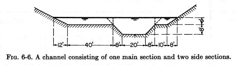
    Channels of Compound Section

  • A natural channel usually consists of a main channel and two side channels.


    Fig. 6-6 (Chow)

  • Let v1, v2, v3, vN, be the mean velocities in the subsections.

  • Let α1, α2, α3, αN, be the α velocity-distribution coefficients in the corresponding subsections.

  • Let β1, β2, β3, βN, be the β velocity-distribution coefficients in the corresponding subsections.

  • Let ΔA1, ΔA2, ΔA3, ΔAN, be the water areas in the corresponding subsections.

  • From continuity:

    v1 = (K1/ΔA1) S1/2

    v2 = (K2/ΔA2) S1/2

    v3 = (K3/ΔA3) S1/2

    vN = (KN/ΔAN) S1/2

    Q = V A = v1 ΔA1 + v2 ΔA2 + v3 ΔA3 + ... + vN ΔAN

    Q = V A = (K1 + K2 + K3 + ... KN) S1/2

    Q = V A = (Σ KN) S1/2

  • Therefore, the mean velocity of the total section is:

    V = (Σ KN) S1/2 / A

  • The velocity-distribution coefficients are:

    α = ∑ v3 ΔA / (V3 A)

    β = ∑ v2 ΔA / (V2 A)

  • Incorporating the velocity into the definitions of velocity-distribution coefficients, the composite values of α and β are, respectively:

    α = [ Σ (αN KN3 / ΔAN2) ] / [(Σ KN)3 / A2 ]

    β = [ Σ (βN KN2 / ΔAN) ] / [(Σ KN)2 / A ]

6.6  DETERMINATION OF NORMAL DEPTH AND VELOCITY


  • The normal depth and velocity can be computed using the Manning equation.


    Fig. 2-2 (Chow)


Example 6-2. Compute the normal depth and velocity of the trapezoidal channel shown above, carrying 400 cfs, with b = 20 ft, z = 2, So = 0.0016, and n = 0.025.

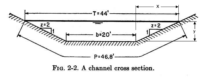
Solution.- The following proportion holds:     z/1 = x/y

From which:    x = zy

T = b + 2x = b + 2zy

A= (1/2) (b + T) y = (1/2) (b + b + 2zy) y = (b + zy) y

P = b + 2 (y2 + z2y2) 1/2 = b + 2y (1 + z2)1/2

R = { [(b/2) + (zy)/2] y}    /   [ (b/2) + y (1 + z2)1/2 ]

Q = (1.486/n) A R2/3 S1/2

(Qn) / (1.486 S1/2) = A R2/3

(Qn) / (1.486 S1/2) = {2[(b/2) + (zy)/2] y}    {[(b/2) + (zy)/2]y }   2/3 / [ (b/2) + y (1 + z2)1/2 ]2/3

[(Qn) / (1.486 S1/2)] [ (b/2) + y (1 + z2)1/2 ]2/3 = 2 {[(b/2) + (zy)/2] y }    5/3

[(Qn) / (2 × 1.486 S1/2)] [ (b/2) + y (1 + z2)1/2 ]2/3 = {[(b/2) + (zy)/2] y }    5/3

[(Qn) / (2 × 1.486 S1/2)]3/2 [ (b/2) + y (1 + z2)1/2 ] = {[(b/2) + (zy)/2] y}    5/2

{ [(b/2) + (zy)/2] y}   5/2 - { [(Qn) / (2 × 1.486 S1/2)]3/2 [(1 + z2)1/2]y}   - [(Qn) / (2 × 1.486 S1/2)]3/2 (b/2) = 0

[(Qn) / (2 × 1.486 S1/2)]3/2 = 771.5

(1 + z2)1/2 = 2.236

{ [(b/2) + (zy)/2] y}    5/2 - [(771.5 × 2.236)y] - 771.5 (b/2) = 0

[(10 + y)y]5/2 - 1725y - 7715 = 0

By trial and error:

yn = 3.36 ft.

An = [(b + zyn) yn] = 89.78 ft.

Vn = Q/An = 400/89.78 = 4.46 fps.


The normal flow depth equation is:

f(y) = { [(b/2) + (zy)/2] y }   5/2 - { [(Qn) / (2 × 1.486 S1/2)]3/2 [(1 + z2)1/2]y}   - [(Qn) / (2 × 1.486 S1/2)]3/2 (b/2) = 0

f(y) = { [(b/2) + (zy)/2] y }   5/2 - { [(Qn) / (2.972 S1/2)]3/2 [(1 + z2)1/2]y}   - [(Qn) / (2.972 S1/2)]3/2 (b/2) = 0

Changing variable to x for simplicity:

f(x) = { [(b/2) + (zx)/2] x }   5/2 - { [(Qn) / (2.972 S1/2)]3/2 [(1 + z2)1/2]x}   - [(Qn) / (2.972 S1/2)]3/2 (b/2) = 0


To solve this equation by trial and error (brute force method), the following simple algorithm is suggested:


  1. Assume x = 0.

  2. Assume Δx = 1.

  3. Increment x:    xo = x + Δx

  4. Calculate f(xo)

  5. Stop when Δx is small enough (calculate output variables).

  6. If f(xo) < 0, return to step 3

  7. If f(xo) > 0, set Δx = 0.1 Δx

  8. Set xo = xo - 9 Δx and return to step 4

Solution by using Newton's approximation:

f(x) = { [(b/2) + (zx)/2] x}   5/2 - { [(Qn) / (2.972 S1/2)]3/2 [(1 + z2)1/2]x}   - [(Qn) / (2.972 S1/2)]3/2 (b/2)

f'(x) = x5/2 (5/2) [(b/2) + (zx)/2] 3/2 (z/2) + [(b/2) + (zx)/2] 5/2 (5/2) x3/2 - [(Qn) / (2.972 S1/2)]3/2 (1 + z2)1/2

f'(x) = (5/4) zx5/2 [(b/2) + (zx)/2]3/2 + (5/2) x3/2 [(b/2) + (zx)/2]5/2 - [(Qn) / (2.972 S1/2)]3/2 (1 + z2)1/2


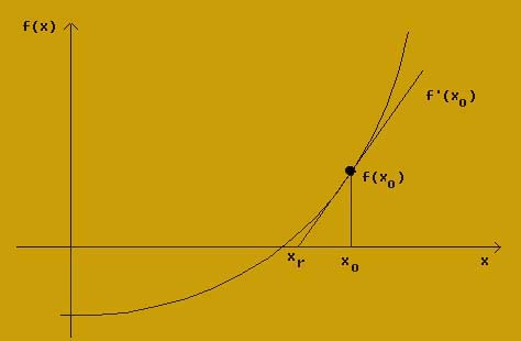
[When the root xr is approached from the left (xo < xr), the slope f'(xo) is positive, f(xo) is negative, and the denominator (xo - xr) is negative].

[When the root xr is approached from the right (xo > xr) (the usual case), the slope f'(xo) is positive, f(xo) is positive, and the denominator (xo - xr) is positive].

Newton's iteration with the root approached from the right.

Thus:

f'(xo) = f(xo) / (xo - xr)

The root is:

xr = xo - f(xo) / f'(xo)

To solve the normal flow depth equation using Newton's approximation, the following algorithm is suggested:


  1. Assume x = 0.

  2. Assume Δx = 1.

  3. Increment x:    xo = x + Δx

  4. Calculate f(xo)

  5. If f(xo) < 0, return to step 3

  6. If f(xo) > 0, then:

  7. Calculate the root:

    xr = xo - [f(xo) / f'(xo)]

  8. Stop when xr - xo is small enough (calculate output variables).

  9. Otherwise, set xo = xr and return to step 7.
6.7  THEORY OF THE MANNING EQUATION


  • In 1891, the Frenchman Flamant attributed to Manning that Chezy C was a function of hydraulic radius:

    C = (1/n) R1/6

    v = C R1/2 S1/2 = (1/n) R2/3 S1/2

    Metric

  • In U.S. customary units (1 m = 3.28 ft):

    v/3.28 = (1/n) (R/3.28)2/3 S1/2

    U.S. customary units

    v = (3.28)1/3 (1/n) R2/3 S1/2

    U.S. customary units

    v = (1.486/n) R2/3 S1/2

    U.S. customary units

  • Williamson plotted in 1951 the Darcy-Weisbach friction factor vs relative roughness:

    fD = 8g/C2 = 0.113 (R/ks)-1/3

    where ks is the linear measure of roughness (grain size).

  • Replacing ks for d84 (diameter for which 84% is finer) and solving for C:

    C = (8g/0.113)1/2 (R/d84)1/6

    C = 1.486 R1/6 / (0.031 d841/6)

  • Therefore:

    n = 0.031 d841/6

    U.S. customary units

  • The general formula for Manning's n as a function of relative roughness R/k and absolute roughness k is:

    n = f (R/k) k1/6

  • Strickler used a constant for f (R/k) = 0.0342, and the median grain size (d50) as the absolute roughness:

    n = 0.0342 d501/6

    U.S. customary units

  • For d50 = 10 ft:    n = 0.050

  • For d50 = 1 ft:    n = 0.034

  • For d50 = 0.1 ft:    n = 0.023

  • For d50 = 0.01 ft:    n = 0.016

  • For d50 = 0.001 ft:    n = 0.011

  • For d50 = 0.0001 ft:    n = 0.007

  • The actual minimum value of n = 0.008 (lucite surface) (Chow).
6.9  COMPUTATION OF FLOOD DISCHARGE: THE SLOPE-AREA METHOD


  • The slope-area method is used to calculate flood discharges when field data regarding wetted cross sections and energy slopes is available.

  • The steps in the application of the slope-area method are the following:

    1. With known upstream and downstream flow areas and hydraulic radius, and average value of Manning n for the reach, compute the conveyances:

      Ku = (1.486/n) Au Ru2/3

      Kd = (1.486/n) Ad Rd2/3

    2. Compute the average conveyance for the reach (the geometric mean):

      K = (KuKd)1/2

    3. Assuming zero velocity-head difference, the first approximation to the energy slope is equal to the fall of water surface elevation divided by the reach length:

      Se = F / L

    4. The first approximation of the discharge is:

      Q = K Se1/2

    5. Compute the velocity heads upstream and downstream:

      hu = αu Vu2/(2g) = αu (Q/Au)2/(2g)

      hd = αd Vd2/(2g)= αd (Q/Ad)2/(2g)

    6. The new energy slope is:

      Se = hf / L = [F + k(hu - hd)] / L

      where k = 1 if the reach is contracting (Vu < Vd), and k = 0.5 is the reach is expanding (Vu > Vd),. The reduction in k accounts for the recovery of the flow during expansion.

    7. The new discharge is:

      Q = K Se1/2

    8. Go back to step 5 and repeat steps 5-7 until the calculated discharge (new discharge) has converged to a constant value (usually 3-4 iterations).

  • Example.

Local man showing water level reached by flood, Kanakumbe, Karnataka, India, December 1991.
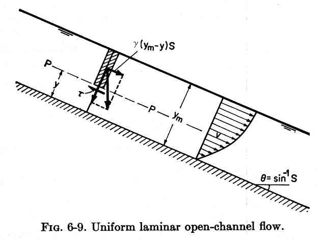
6.10  UNIFORM SURFACE FLOW


  • Overland flow over a surface can be described as uniform surface flow.

  • This type of flow is also referred to as sheet flow, when the depth is small compared to the width.

  • The flow may be laminar or turbulent.

  • If the flow depth is small, viscosity dominates and the flow is laminar.


    Fig. 6-9 (Chow)

  • The acting shear stress is:

    τ = γ (ym - y) S

  • According to Newton's law of viscosity, the resisting shear stress is:

    τ = μ (dv/dy)

  • Therefore:

    μ (dv/dy) = γ (ym - y) S

    dv = (γ/μ) (ym - y) S dy

  • But:

    γ = ρg

    μ = ρν

  • Then:

    dv = (gS/ν) (ym - y) dy

  • Integrating:

    v = dv = (gS/ν) (ym - y) dy

    v = (gS/ν) [ (ymy) - (y2/2) ] + C

  • For v = 0: y = 0. Then C = 0.

  • The velocity-depth function is:

    v = (gS/ν) [ (ymy) - (y2/2) ]

  • Thus, the velocity of uniform sheet flow has a parabolic distribution.

  • Integrate the velocity distribution to find the rating:

    q = vdy = (gS/ν) [ (ymy) - (y2/2) ] dy

    (Between the limits of 0 and ym)

    q = (gS/ν) [ (ym3/2) - (ym3/6) ]

    (Between the limits of 0 and ym)

    q = (gS/ν) [ (1/3)ym3 ]

    q = [ (gS)/(3ν) ] ym3 = CL ym3

    CL = (gS)/(3ν)

  • Note that in laminar flow the exponent of the rating is 3, and the rating is a function of the internal friction ν

  • The mean velocity is:

    v = q/ym = [(gS)/(3ν)] ym2 = CL ym2

  • The turbulent flow rating for sheet flow (Manning friction) is:

    q = v ym = (1.486/n) S1/2 ym5/3

  • Note that in turbulent flow (Manning) the exponent of the rating is 5/3.

  • The turbulent flow rating for sheet flow (Chezy friction) is:

    q = v ym = C S1/2 ym3/2

  • Note that in turbulent flow (Chezy) the exponent of the rating is 3/2.

  • Note that for sheet flow, the exponent of the rating varies between 3/2-5/3 (turbulent) and 3 (laminar).

  • A value of 2 is mixed laminar-turbulent.

  • The Vedernikov number is:

    V = (β - 1)U/(gD)1/2

    where β is the exponent of the rating and U is the mean velocity.

  • For β = 3 (laminar):

    V = 2U/(gD)1/2 = 2 F

  • It follows that in laminar flow, the flow is unstable (V = 1) when F = 0.5.

  • For β = 3/2 (Chezy turbulent):

    V = (1/2)U/(gD)1/2 = (1/2) F

  • In turbulent Chezy flow, the flow is unstable (V = 1) when F = 2.

  • For β = 5/3 (Manning turbulent):

    V = (2/3)U/(gD)1/2 = (2/3) F

  • In turbulent Manning flow, the flow is unstable (V = 1) when F = 3/2.

 
140404