CIVE 530 - OPEN-CHANNEL HYDRAULICS

LECTURE 15: HEC-RAS, Users Manual, Chapter 4, Example Application

STARTING A NEW PROJECT

  • This chapter provides an example application of how to perform steady flow water surface profile calculations with HEC-RAS.

  • You are taken through a step-by-step procedure of how to enter data, perform calculations, and view the results.

  • Contents

    • Starting a New Project

    • Entering Geometric Data

    • Entering Steady Flow Data

    • Performing the Hydraulic Calculations

    • Viewing Results

    • Printing Graphics and Tables

    • Exiting the Program

  • To begin this example, let's first start the HEC-RAS program.

  • Double click the HEC-RAS icon in Windows.

  • The main window should appear as shown in Figure 4.1 (except yours will be blank the first time you start the program).


    Figure 4.1   The HEC-RAS Main Window.


  • The first step in developing an HEC-RAS application is to start a new project.

  • Go to the File menu on the main window and select New Project.

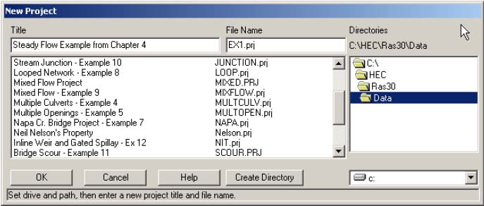
  • The New Project window should appear as shown in Figure 4.2 (except the title and file name fields will be blank when it first comes up).


    Figure 4.2   The HEC-RAS New Project Window.


  • First set the drive (e.g., C:) and the directory that you would like to work in.

  • Next enter the project title and filename as shown in Figure 4.2.

  • Once you have entered the information, press the OK button to have the data accepted.


ENTERING GEOMETRIC DATA

  • The next step in developing a steady flow model with HEC-RAS is to enter the geometric data.

  • This is accomplished by selecting Geometric Data from the Edit menu on the HEC-RAS main window.

  • Once this option is selected, the geometric data window will appear (except yours will be blank when you first bring it up) (Figure 4.3).
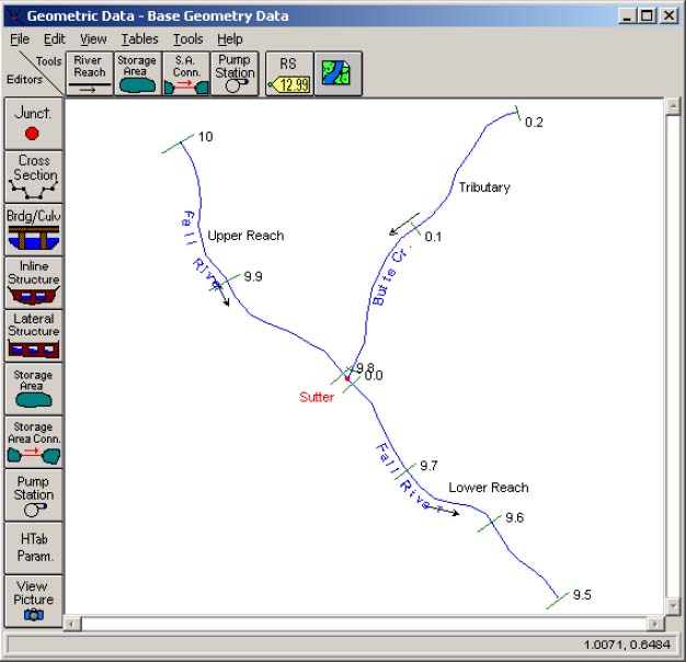

    Figure 4.3   The HEC-RAS Geometric data window with example river schematic.


Drawing the schematic of a river system
  • In this example we are going to develop a two-river (three hydraulic reaches) system as shown in Figure 4.3.

  • Draw the river system schematic by performing the following steps:

    1. Click the River Reach button on the geometric data window.

    2. Move the mouse pointer over to the drawing area and place the pointer at the location in which you would like to start drawing the

    3. first reach.

    4. Press the left mouse button once to start drawing the reach.

      Move the mouse pointer and continue to press the left mouse button to add additional points to the line segment.

      To end the drawing of the reach, double click the left mouse button and the last point of the reach will be placed at the current mouse pointer location.

      All reaches must be drawn from upstream to downstream (in the positive flow direction), because the program assumes this to be true.

    5. Once the reach is drawn, the interface will prompt you to enter an identifier for the River name and the Reach name.

      The River identifier can be up to 32 characters, while the reach name is limited to 12 characters.

      In this example, there is one river named Fall River and another one named Butte Cr.

      Fall river contains two hydraulic reaches, which are labeled Upper Reach and Lower Reach.

      Butte Cr. has been entered as a single hydraulic reach, and the reach name is Tributary.

    6. Repeat steps one through four for each reach.

      After you enter the identifiers for Butte Cr., you will also be prompted to enter an identifier for the junction.

      Junctions in HEC-RAS are locations where two or more reaches join together or split apart.


    Figure 4.3   The HEC-RAS Geometric data window with example river schematic.


  • Once you have finished drawing in the river system, there are several options available for editing the schematic.

  • These options include: change name, move object (objects are labels, junctions, and points in the reaches), add points to a reach, remove points from a reach, delete a reach, and delete a junction.

  • The editing features are located under the Edit menu on the Geometric Data window.

  • Note: when you first draw your schematic there will not be any tic marks representing cross sections as shown in Figure 4.3. The tic marks only show up after you have entered cross sections.


Entering Cross Section Data

  • The next step is to enter the cross section data.

  • This is accomplished by pressing the Cross Section button on the Geometric Data window (Figure 4.3).

  • Once this button is pressed, the Cross Section Data editor will appear as shown in Figure 4.4 (except yours should be blank).

  • To enter cross section data do the following:

    1. Select a River and a Reach to work with.

      For this example start with the Fall River, Upper Reach.

    2. Go to the Options menu and select Add a new Cross Section.

      An input box will appear to prompt you to enter a river station identifier for the new cross section.

      The identifier does not have to be the actual river station, but it must be a numeric value.

      The numeric value describes where this cross section is located in reference to all the other cross sections within the reach.

      Cross sections are located from upstream (highest river station) to downstream (lowest river station). For this cross section enter a value of 10.0.

    3. Enter all of the data for this cross section as it is shown in Figure 4.4.
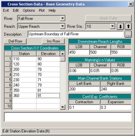

      Figure 4.4   Cross section data editor with data example.


    4. Once all the data are entered press the Apply Data button.

      This button is used to tell the interface that you want the data to be accepted into memory.

      This button does not save the data to your hard disk, which can only be accomplished from the File menu on the Geometric Data window.

    5. Plot the cross section to visually inspect the data.

      This is accomplished by pressing the Plot Cross Section option under the Plot menu on the Cross Section Data Editor.

      The cross section should look the same as that shown in Figure 4.5.
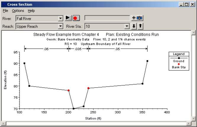

    Figure 4.5   Cross section plot for river mile 10.0 of Fall Creek.


  • In general, the five steps listed would be repeated for every cross section that is entered.

  • In order to reduce the amount of data entry for this example, the current cross section will be copied and adjusted to represent other cross sections within the river system.


  • The following steps should be followed to copy the current cross section:

    1. Go to the Options menu on the Cross Section Data Editor and select Copy Current Cross Section.

      An input box will appear to prompt you to select a river and a reach, and then enter a river station for the new cross section.

      For this example, keep the river and reach as Fall River and Upper Reach, then enter a new river station of 9.9.

      Press the OK button and the new cross section will appear in the editor.

    2. Change the cross section description to "River Mile 9.9 of Fall River."

    3. Adjust all the elevations of the cross section by -0.5 feet.

      This is accomplished by selecting the Adjust Elevations feature from the Options menu on the Cross Section Data Editor.

    4. Adjust the cross section stationing to reduce the overbanks by 10%.

      This is accomplished by selecting the Adjust Stations feature from the Options menu on the Cross Section Data Editor, then select Multiply by a Factor.

      When the input box appears for this option, three data entry fields will be available to adjust the stationing of the left overbank, channel, and the right overbank separately.

      Enter values of 0.90 for the right and left overbanks, but leave the main channel field blank.

      This will reduce the stationing of both overbanks by 10%, but the main channel will not be changed.

    5. Downstream reach lengths remain the same for this cross section.

    6. Press the Apply Data button.

    7. Plot the cross section to visually inspect it.

  • These seven steps should be repeated to enter all the data for Fall River (Upper and Lower Reach).

  • The necessary adjustments are listed in Table 4.1.


    Table 4.1 Cross section adjustments for duplicating sections
    Cross sectionAdjusted elevation Adjusted stationing Downstream reach lengths
    Reach River Sta.Left O.B. Channel Right O.B. Left O.B. Channel Right O.B.
    Upper 9.8 -0.4 0.80 - 0.80 0 0 0
    Lower 9.79 -0.1 1.20 1.20 1.20 500 500 500
    Lower 9.7 -0.5 1.20 1.20 1.20 500 500 500
    Lower 9.6 -0.3 - - - 500 500 500
    Lower 9.5 -0.2 - - - 0 0 0


  • Perform the cross section duplications in the order that they are listed in the table.

  • Make sure to change the description of each cross section, and also press the Apply Data button after making the adjustments for each cross section.


  • This completes all the cross section data for Fall River (upper and Lower reach).

  • Now let's work on entering the data for the Butte Creek tributary.

  • To enter the first cross section in the Butte Creek tributary do the following:

    1. Go to the River text box on the Cross Section Data Editor and select the Butte Cr. river.

      The Reach of "Tributary" will automatically be selected since it is the only reach in Butte Creek.

    2. Select Add a new Cross Section from the Options menu.

      When the popup box appears to prompt you to enter a new river station, enter a value of 0.2.

    3. Enter all the data for this cross section as shown in Figure 4.6.
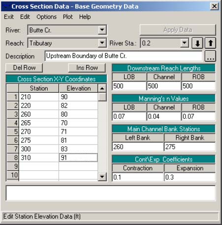

      Figure 4.6   Cross Section Editor with river mile 0.2 of Butte Creek.


    4. Once all the data are entered for this section, press the Apply Data button.

    5. Plot the cross section to inspect the data.


  • There are two other cross sections that need to be developed for the Butte Creek tributary.

  • These two cross sections will be developed by duplicating the cross section that you just entered, and then adjusting the elevations and stationing.

  • The necessary adjustments are listed in Table 4.2.


    Table 4.2 Cross section adjustments for Butte Creek sections
    Cross sectionAdjusted elevation Adjusted stationing Downstream reach lengths
    Reach River Sta.Left O.B. Channel Right O.B. Left O.B. Channel Right O.B.
    Butte Creek 0.1 -0.6 - - - 500 500 500
    Butte Creek 0.0 -0.3 - - - 0 0 0


  • Perform the cross section adjustments in the order that they are listed in the table.

  • Make sure to change the description of each cross section and press the Apply Data button after editing is complete.


  • Now that all of the cross section data are entered, save the data to a file before continuing.

  • Saving the data to a file is accomplished by selecting the "Save Geometry Data As" option from the File menu on the Geometric Data window.

  • After selecting this option you will be prompted to enter a Title for the geometric data.

  • Enter "Base Geometry Data" for this example, then press the OK button.

  • A file name is automatically assigned to the geometry data based on what you entered for the project filename.


Entering Junction Data

  • The next step is to enter the junction data. Junction data consist of a description, and reach lengths across the junction.

  • In this example there is only one junction, which is labeled Sutter.

  • To enter Junction data, press the Junction button on the Geometric Data window.

  • Enter the junction data as shown in Figure 4.7.
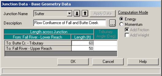

    Figure 4.7   Junction Data Editor, with Sutter junction data.


  • Reach lengths across the junction are entered in the junction editor, rather than in the cross section data.

  • This allows for the lengths across very complicated confluences (i.e., flow splits) to be accommodated.

  • In the cross section data, the reach lengths for the last cross section of each reach should be left blank or set to zero.


  • In this example the energy equation will be used to compute the water surface profile through the junction.

  • If the momentum equation is selected, then an angle can be entered for one or more of the reaches flowing into or out of a junction.

  • The momentum equation is set up to account for the angle of the flow entering the junction.


  • Once you have all of the data entered for the junction, apply the data and close the window by pressing the OK button.


Saving the Geometry Data

  • At this point in the example, all of the geometric data has been entered.

  • Before we continue with the example, you should save the geometric data to the hard disk.

  • Since the data have already been saved once, you simply have to select Save Geometry Data from the File menu on the Geometric Data window.

  • We can now go on to enter the Steady Flow data.


ENTERING STEADY FLOW DATA

  • The next step in developing the required data to perform steady flow water surface profile calculations is to enter the steady flow data.

  • To bring up the steady flow data editor, select Steady Flow Data from the Edit menu on the HEC-RAS main window.

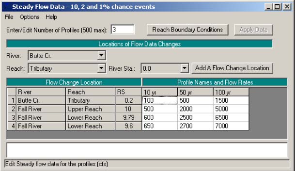
  • The Steady Flow Data editor should appear as shown in Figure 4.8.


    Figure 4.8   Steady Flow Data Editor, with example problem data.


  • The first piece of data to enter is the number of profiles to be calculated.

  • For this example, enter "3" as shown in Figure 4.8.

  • The next step is to enter the flow data.

  • Flow data are entered from upstream to downstream for each reach.

  • At least one flow rate must be entered for every reach in the river system.

  • Once a flow value is entered at the upstream end of a reach, it is assumed that the flow remains constant until another flow value is encountered within the reach.

  • Additional flow values can be entered at any cross section location within a reach.


  • In this example, flow data will be entered at the upstream end of each reach.

  • An additional flow change location will be entered at river mile 9.6 of the Fall River in the Lower Reach.

  • To add an additional flow change location into the table, first select the Fall River, Lower Reach from the Reach list box.

  • Next, select the desired river station location (9.6 in this example) from the River Sta. list box.

  • Finally, press the Add a Flow Change Location button.

  • The new flow location should appear in the table.

  • Now enter all of the flow data into the table as shown in Figure 4.8.

  • Profile labels will automatically default to "PF#1," "PF#2," etc.

  • You can change these labels to whatever you want. In this example they have been changed to "10 yr," "50 yr," and "100 yr," to represent the statistical return period of each of the events being modeled.


  • The next step is to enter any required boundary conditions.

  • To enter boundary conditions, press the Enter Boundary Conditions button at the top of the Steady Flow Data editor.

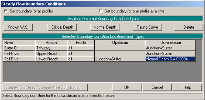
  • The boundary conditions editor will appear as shown in Figure 4.9, except yours will be blank the first time you open it.


    Figure 4.9   Steady Flow Boundary Conditions.


  • Boundary conditions are necessary to establish the starting water surface at the ends of the river system.

  • A starting water surface is necessary in order for the program to begin the calculations.

  • In a subcritical flow regime, boundary conditions are only required at the downstream ends of the river system.

  • If a supercritical flow regime is going to be calculated, boundary conditions are only necessary at the upstream ends of the river system.

  • If a mixed flow regime calculation is going to be made, then boundary conditions must be entered at all open ends of the river system.


  • The boundary conditions editor contains a table listing every river and reach.

  • Each reach has an upstream and a downstream boundary condition.

  • Connections to junctions are considered internal boundary conditions.

  • Internal boundary conditions are automatically listed in the table, based on how the river system is connected in the geometric data editor.

  • The user is only required to enter the necessary external boundary conditions.


  • In this example, it is assumed that the flow is subcritical throughout the river system.

  • Therefore, it is only necessary to enter a boundary condition at the downstream end of the Fall River, Lower Reach.

  • Boundary conditions are entered by first selecting the cell in which you wish to enter a boundary condition.

  • Then the type of boundary condition is selected from the four available types listed above the table.

  • The four types of boundary conditions are:

    • Known water surface elevations

    • Critical depth

    • Normal depth

    • Rating curve

  • For this example, use the normal depth boundary condition.

  • Once you have selected the cell for the downstream end of Fall River, Lower Reach, press the Normal Depth button.

  • A pop up box will appear requesting you to enter an average energy slope at the downstream end of the Fall River.

  • Enter a value of 0.0004 (ft/ft) then press the Enter key.

  • This completes all of the necessary boundary condition data.

  • Press the OK button on the Boundary Conditions form to accept the data.


  • The last step in developing the steady flow data is to save the data to a file.

  • To save the data, select the Save Flow Data As option from the File menu on the Steady Flow Data Editor.

  • A pop up box will prompt you to enter a description of the flow data.

  • For this example, enter "10, 2, and 1% chance events."

  • Once the data are saved, you can close the Steady Flow Data Editor.


PERFORMING THE HYDRAULIC CALCULATIONS

  • Now that all of the data have been entered, we can calculate the steady water surface profiles.

  • To perform the simulations, go to the HEC-RAS main window and select Steady Flow Analysis from the Run menu.

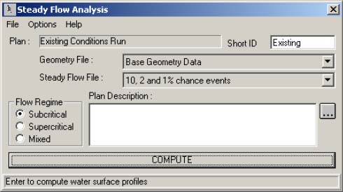
  • The Steady Flow Analysis window should appear as shown in Figure 4.10, except yours will not have any plan titles yet.


    Figure 4.10   Steady Flow Analysis Simulation Window.


  • The first step is to put together a Plan.

  • The Plan defines which geometry and flow data are to be used, as well as providing a title and short identifier for the run.

  • To establish a plan, select New Plan from the File menu on the Steady Flow Analysis window.

  • Enter the plan title as "Existing Conditions Run" and then press the OK button.

  • You will then be prompted to enter a short identifier.

  • Enter a title of "Existing" in the Short ID box.


  • The next step is to select the desired flow regime for which the model will perform calculations.

  • For this example we will be performing Subcritical flow calculations only.

  • Make sure that Subcritical is the selected flow regime.

  • Additional job control features are available from the Options menu bar, but none are required for this example.

  • Once you have defined a plan and set all the desired job control information, the plan information should be saved.

  • Saving the plan information is accomplished by selecting Save Plan from the File menu of the Steady Flow Analysis window.


  • Now that everything has been set, the steady flow computations can be performed by pressing the Compute button at the bottom of the Steady Flow Simulation window.

  • Once the compute button has been pressed, a separate window will appear showing you the progress of the computations.

  • Once the computations have been completed, the computation window can be closed by double clicking the upper left corner of the window.

  • At this time the Steady Flow Simulation window can also be closed.


VIEWING THE RESULTS

  • Once the model has finished all of the computations successfully, you can begin viewing the results.

  • Several output options are available from the View menu bar on the HEC-RAS main window.

  • These options include:

    • Cross section plots

    • Profile plots

    • General Profile Plot

    • Rating curves

    • X-Y-Z Perspective Plots

    • Detailed tabular output at a specific cross section (cross section table)

    • Limited tabular output at many cross sections (profile table)


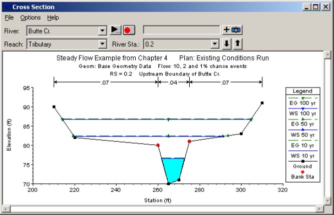
  • Let's begin by plotting a cross section.

  • Select Cross Sections from the View menu bar on the HEC-RAS main window.

  • This will automatically bring up a plot of the first cross section in Butte Cr., as shown in Figure 4.11.


    Figure 4.11   Cross section plot for example application.


  • Any cross section can be plotted by selecting the appropriate river, reach, and river station from the list boxes at the top of the cross section plot window.

  • The user can also step through the plots by using the up and down arrow buttons.

  • Several plotting features are available from the Options menu bar on the cross section plot window.

  • These options include: zoom in; zoom out; selecting which plans, profiles and variables to plot; and control over lines, symbols, labels, scaling, and grid options.


  • Select different cross sections to plot and practice using some of the features available under the Options menu bar.


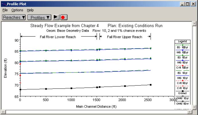
  • Next let's plot a water surface profile.

  • Select Water Surface Profiles from the View menu bar on the HEC-RAS main window.

  • This will automatically bring up a water surface profile plot for the first reach, which is Butte Cr. in our example.

  • To plot more than one reach, select Reaches from the Options menu bar on the profile plot.

  • This option brings up a list of available rivers and reaches from which to choose.

  • Select the Upper and Lower reaches of the Fall river.

  • This should give you a profile plot as shown in Figure 4.12.


    Figure 4.12   Profile plot for example application.


  • Plot the additional profiles that were computed and practice using the other features available under the Options menu bar on the profile plot.


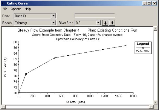
  • Now let's plot a computed rating curve.

  • Select Rating Curves from the View menu on the HEC-RAS main window.

  • A rating curve based on the computed water surface profiles will appear for the first cross section in Butte Cr., as shown in Figure 4.13.


    Figure 4.13   Computed rating curve for example application.


  • You can look at the computed rating curve for any location by selecting the appropriate river, reach, and river station from the list boxes at the top of the plot.

  • Plotting options similar to the cross section and profile plots are available for the rating curve plots.

  • Plot rating curves for various locations and practice using the available plotting options.


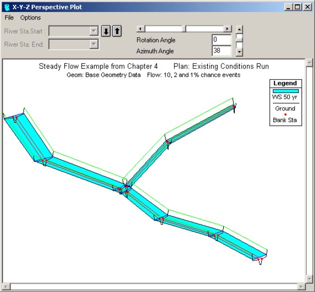
  • Next look at an X-Y-Z Perspective Plot of the river system.

  • From the View menu bar on the HEC-RAS main window, select X-Y-Z Perspective Plots.

  • A multiple cross section perspective plot should appear on the screen.

  • From the Options menu, select Reaches.

  • A pop up window will appear allowing you to select which rivers and reaches you would like to have on the plot.

  • Press the Select All button and then the OK button.

  • Also, under the Options menu, select the Profiles option.

  • Select profile two to be plotted from the three available profiles.

  • Once you have selected these options, and X-Y-Z perspective plot should appear on the screen, similar to the one shown in Figure 4.14.

  • Try rotating the perspective view in different directions, and select different reaches to look at.


    Figure 4.14   X-Y-Z perspective plot for all three river reaches.


  • Now let's look at some tabular output.

  • Go to the View menu bar on the HEC- RAS main window.

  • There are two types of tables available, a detailed output table and a profile summary table.

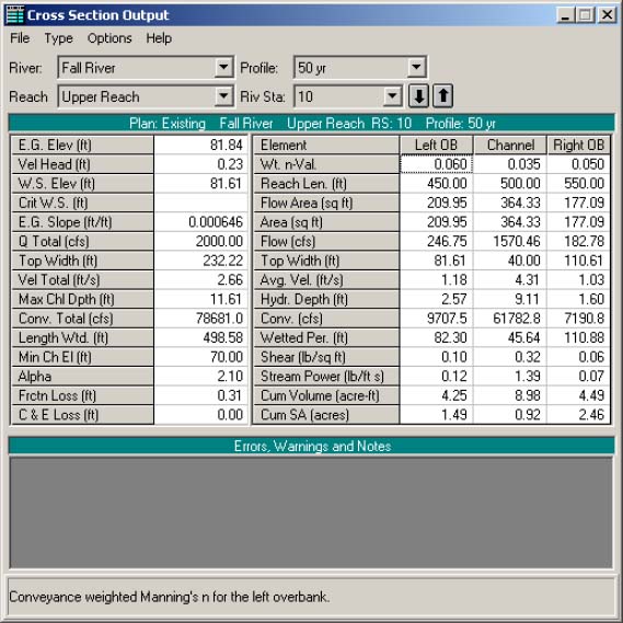
  • Select Detailed Output Tables to get the first table to appear.

  • The table should look like the one shown in Figure 4.15.

  • This table shows detailed hydraulic information at a single cross section. Other cross sections can be viewed by selecting the appropriate reach and river mile from the table.


    Figure 4.15   Detailed tabular output at a cross section.


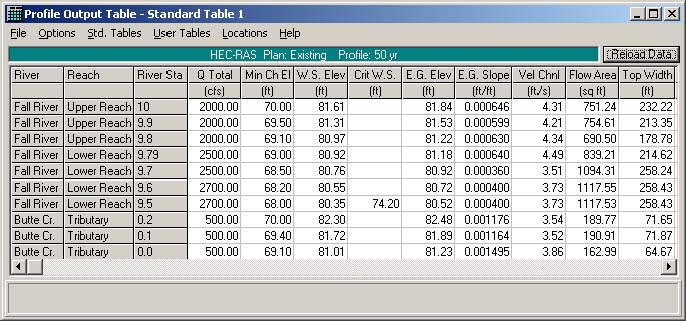
  • Now bring up the profile summary table.

  • This table shows a limited number of hydraulic variables for several cross sections.

  • There are several types of profile tables listed under the Std. Tables menu bar of the profile table window.

  • Some of the tables are designed to provide specific information at hydraulic structures (e.g., bridges and culverts), while others provide generic information at all cross sections.

  • An example of this type of table is shown in Figure 4.16.


    Figure 4.16   Tabular output in profile format.


PRINTING GRAPHICS AND TABLES

  • All of the plots and tables can be sent directly to a printer/plotter or passed through the Windows clipboard to another program (e.g., a word processor).

  • The printer or plotter that gets used is based on what you currently have selected as the default printer for Windows.

  • The user has the ability to change many of the default printer settings (e.g., portrait to landscape) before printing occurs.


Sending graphics directly to the printer

  • To send a graphic to the printer/plotter, do the following:

    1. Display the graphic of interest (cross section, profile, rating curve, or river system schematic) on the screen.

    2. Using the available options (scaling, labels, grid, etc.), modify the plot to be what you would like printed out.

    3. Select Print from the File menu of the displayed graphic.

      Once Print is selected, a Printer Options window will appear, giving the user the opportunity to change any of the default printer settings.

      Once you have the print settings the way you want them, press the Print button on the Printer Options window and the plot will automatically be sent to the Windows Print Manager.

      From that point the Windows Print Manager will control the printing.


Sending graphics to the Window clipboard

  • To pass a graphic to the Windows clipboard and then to another program, do the following:

    1. Display the graphic of interest on the screen.

    2. Using the available options, modify the plot to be what you want it to look like.

    3. Select Copy to Clipboard from the File menu of the displayed graphic.

      The plot will automatically be sent to the Windows clipboard.

    4. Bring up the program that you want to pass the graphic into (e.g., word processor).

      Select Paste from the Edit menu of the receiving program.

      Once the graphic is pasted in, it can be resized to the desired dimensions.


Sending tables directly to the printer

  • To send a table to the printer, do the following:

    1. Bring up the desired table from the tabular output section of the program.

    2. Select Print from the File menu of the displayed table.

      Once the Print option is selected, a Printer Options window will appear.

      Set any print options that are desired then press the Print button.

      This will send the entire table to the Windows Print Manager

      From this point the Windows Print Manager will control the printing of the table.


  • The profile type of table allows you to print a specific portion of the table, rather than the whole thing.

  • If you desire to only print a portion of the table, do the following:

    1. Display the desired profile type table on the screen.

    2. Using the mouse, press down on the left mouse button and highlight the area of the table that you would like to print.

      To get an entire row or column, press dPortions of the profile table can be sent to the clipboard in the same manner as sending them to the printer. Practice sending graphics and tables to the printer and the clipboard with the example data set that you currently have open. own on the left mouse button while moving the pointer across the desired row or column headings.

    3. Select Print from the File menu of the displayed table.

      Only the highlighted portion of the table and the row and column headings will be sent to the Windows Print Manager.


Sending tables to the Window clipboard

  • To pass a table to the Windows clipboard and then to another program, do the following:

    1. Display the desired table on the screen.

    2. Select Copy to Clipboard from the File menu of the displayed table.

    3. Bring up the program that you want to pass the table into.

      Select Paste from the Edit menu of the receiving program.


  • Portions of the profile table can be sent to the clipboard in the same manner as sending them to the printer.

  • Practice sending graphics and tables to the printer and the clipboard with the example data set that you currently have open.


EXITING THE PROGRAM

  • Before you exit the HEC-RAS software, make sure you have saved all the data.

  • This can be accomplished easily by selecting Save Project from the File menu on the HEC-RAS main window.

  • Any data (geometric, flow, and plan data) that have not been saved will automatically be saved for you.


  • To exit the HEC-RAS software, select Exit from the File menu of the HEC- RAS main window.

  • The program will prompt you to save the project if the data have not been saved previously.

 
051020