|
|
CIVE 445 - ENGINEERING HYDROLOGY
CHAPTER 2D: BASIC HYDROLOGIC PRINCIPLES, RUNOFF
|
- Surface runoff, or simply runoff, refers to all waters flowing on the surface of the earth, in:
- Overland flow
- Rill flow
- Gully flow
- Streamflow
- River flow
- Rivers carry their flow into the ocean, completing the hydrologic cycle.
- Runoff is expressed in terms of volume or flow rate.
- The local flow rate can be integrated over a period of time to give the accumulated runoff volume.
- Runoff is commonly expressed in depth units, i.e., the runoff volume spread uniformly over the catchment area.
- Runoff is also expressed as:
- peak flow per unit drainage area,
- peak flow per unit area per unit rainfall intensity (C),
- peak flow per unit runoff depth, or
-
peak flow per unit drainage area per unit runoff depth.
Runoff components
- Runoff has three sources:
- surface,
- interflow,
- groundwater.
- Surface flow is also called direct runoff.
- Direct runoff can produce large flow concentrations in a relatively short period of time.
- Direct runoff is responsible for floods.
- Interflow is mostly vertical movement of water in the unsaturated portion of the soil profile.
- Groundwater flow takes place below the water table.
- Groundwater is a characteristically slow process.
- Runoff is always moving from higher to lower potential.
- Because water table is almost horizontal,
groundwater flow is almost horizontal.
- Groundwater flow intercepts surface flow in streams and rivers.
- Most groundwater flow is converted to surface runoff before it reaches the ocean.
- Only about 2% of the water in the hydrologic cycle is unaccounted for as either evaporation or surface runoff.
- This unaccounted portion is referred to as
deep percolation, and is commonly neglected in water balance studies.
Stream types and baseflow
- Streams can be grouped into three types:
- perennial,
- ephemeral,
- intermittent.
- Perennial streams are those that always have flow.
- During dry weather, the flow of perennial
streams is baseflow, consisting mostly of groundwater flow.
- Streams that feed from groundwater are called effluent streams.
- Perennial and effluent streams are typical of subhumid and humid regions.
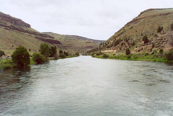
A perennial stream: The Deschutes river, central Oregon.
|
|
- Ephemeral streams flow only in direct response to precipitation.
- Ephemeral streams do not intercept groundwater and have no baseflow.
- Ephemeral streams usually contribute to groundwater by seepage through their porous channel beds.
- Streams that feed groundwater are called influent streams.
- Channel abstractions from influent streams
are called channel transmission losses.
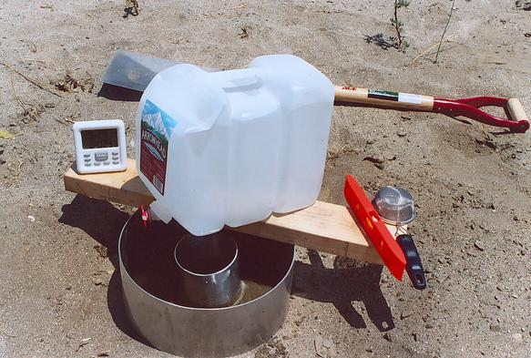
Equipment to measure field hydraulic conductivity.
|
|
- Ephemeral and influent streams are typical of semiarid and arid regions.
- Intermittent streams are those that have intermediate properties, behaving as either perennial or ephemeral, depending on the season.
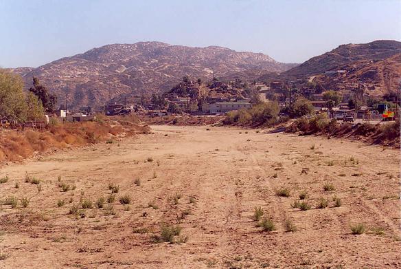
An ephemeral stream: Tecate Creek at El Descanso, Baja California.
|
|
- Baseflow estimates are important in yield hydrology.
- In flood hydrology, knowledge of baseflow is necessary to separate
direct and indirect runoff.
- Baseflow is a measure of indirect runoff.
Antecedent moisture
- Surface runoff depends on antecedent moisture.
- The more antecedent moisture, the less surface runoff.
- The most widely used method for antecedent moisture is the NRCS,
which uses uses the Antecedent Moisture Condition (AMC)
to characterize antecedent moisture:
- I (dry),
- II (average) and
- III (wet).
- Runoff from I is less than II, and II is less than III.
Rainfall-runoff relations
- Rainfall is easier to measure than runoff.
- From an engineering standpoint, the quantity of runoff is more important that the quantity of rainfall.
- Runoff is assessed through rainfall-runoff relations.
- A basic linear model of rainfall-runoff is the following:

Fig. 2-25
|
|
- SCS runoff curve number method is a rainfall-runoff model that has a nonlinear fit to the data.
- Method is conceptual based on empirical data.
Runoff concentration
- Assume that a storm falling on a given catchment produces a uniform effective rainfall intensity over the entire catchment.
- In such case, surface runoff will concentrate at the catchment outlet, provided the effective rainfall is sufficiently long.
- The flow rate at the outlet increases gradually from zero to a constant maximum, or equilibrium value.
- Surface runoff has concentrated at the catchment outlet.
- The time to achieve the maximum discharge is referred to as the time of concentration.
- The equilibrium flow rate is calculated as follows:
where:
- Qe = equilibrium flow rate, in L/s.
- Ie = effective rainfall intensity, in mm/hr.
- A = catchment area, in ha.
- There are three types of catchment flow:
- superconcentrated,
- concentrated,
- subconcentrated.
- Superconcentrated and concentrated flows are typical of small catchments (the rational method).
- Subconcentrated flows are typical of midsize (and large) catchments (the unit hydrograph).
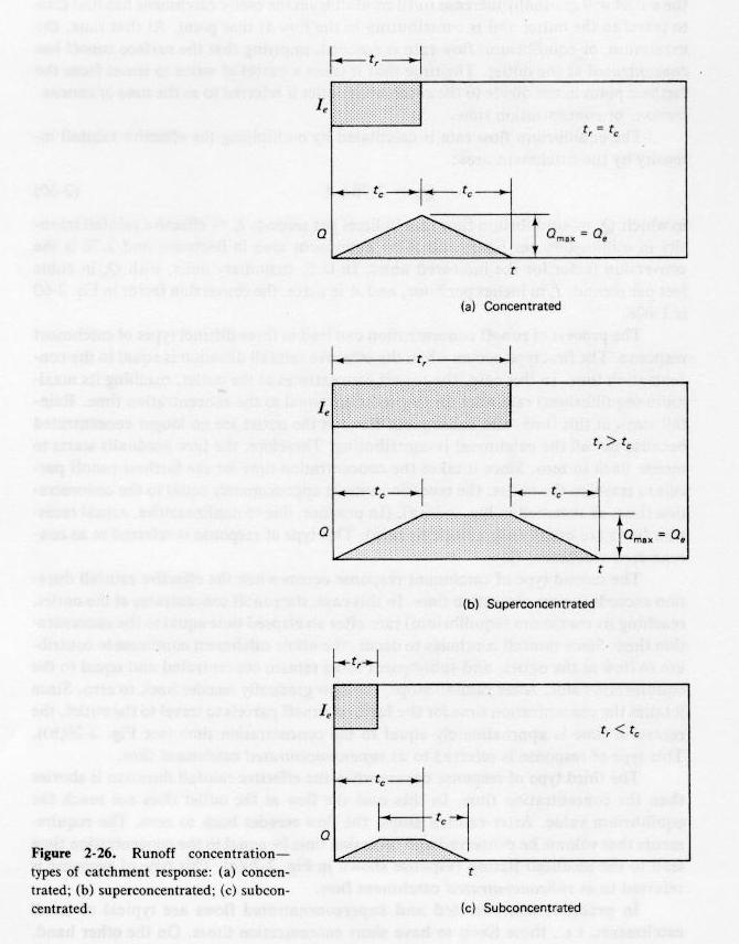
Fig. 2-26
|
|
Time of concentration
- It is the time it takes a parcel of water to travel
from the farthest point in the catchment divide to the outlet.
- It is a function of runoff rate.
- Most formulas for time of concentration are empirical; there are some theoretical (kinematic wave).
- The Manning equation is also used to estimate time of concentration.
- The speed of travel of unsteady flow is usually larger (by 33% to 67%) than the speed of travel of steady flow.
- Time of concentration is essentially unsteady.
- Uncertainties in flow rate have blurred the distinction between steady and unsteady velocities in open-channel flow.
- The Kirpich formula is the most popular formula for time of concentration:
|
tc = 0.06628 L0.77 / S0.385
|
where:
- tc = time of concentration, in hr.
- L = catchment length, in km.
- S = catchment slope, in m/m.
- The Hathaway formula is also popular:
|
tc = 0.606 (Ln)0.467 / S0.234
|
where:
- n = roughness factor (similar to Manning's).
Runoff diffusion and streamflow hydrographs
- Actual catchment response is more complex than that which
could be attributed solely to runoff concentration.
- Rainfall is not uniformly distributed over space,
creating nonuniformities which show as diffusion.
- The runoff process is subject to convection and
diffusion.
- Convection is properly runoff concentration.
- Diffusion is the mechanism acting to spread the flows in time and space.
- Diffusion reduces the flow levels below those that could be attained by convection only.
- Diffusion acts to smooth out catchment response.
- The resulting hydrograph is usually continuous.
- Typical storm hydrographs are shown below.

Fig. 2-27
|
|
Flow in stream channels
- The following properties are used to describe stream channels:
- Cross-sectional dimensions: width, depth, area
- Cross-sectional shape
- Longitudinal slope
- Boundary friction
- Channel top widths vary widely, from a few meters to several kilometers.
- Mean flow depths vary from a fraction of a meter to as high as 60 m for very large rivers such as the Amazon.
- Width-to-depth (aspect) ratios vary from about 10 to more than 100.
- Water surface slope or energy slope is used as a measure of longitudinal channel slope.
- The longer the reach, the more accurate the calculation of channel slope.
- Boundary friction can be due to skin or form friction.
- Since most rivers have aspect ratios greater than 10, boundary friction is synonymous with bottom friction.
Uniform-flow formulas
- The Manning or Chezy formulas are used to calculate uniform flow in stream channels:
where:
- V= mean velocity, m/s.
- R= hydraulic radius, m.
- S = channel slope, in m/m.
- Values of n vary from 0.024 to 0.079 in natural channels (measured by USGS):
See manningsn.sdsu.edu
- Values of n vary from 0.1 to 0.2 in flood plains:
See manningsn2.sdsu.edu
- The Chezy formula is also popular:
where:
- C = Chezy coefficient, varying from 79 to 11 m1/2/s.
- More typical values of Chezy C are in the range from 40 to 70 m1/2/s.
- Unlike the Manning equation, the Chezy can be made dimensionless by dividing the coefficient by the square root of the gravitational
acceleration.
- Despite this theoretical appeal, the Manning equation has had wider acceptance in practice.
- This is attributed to the fact that the Chezy coefficient has a tendency to vary with the hydraulic radius, such that:
- This implies that Manning's n is a constant.
- Experience has shown, however, that n varies with stage and discharge in natural channels.
River stages
- At any point, river stage is the elevation of the water surface above a given datum.
- River stages vary with flow rate.
- Flow rates can be grouped into:
- Low flow is typical of the dry season, and consists mostly of baseflow.
- High flow occurs during the wet season, and contributions are due primarily to surface runoff.
- Average flow occurs in midseason.
- The study of low flows is necessary to determine minimum flow rates below which a certain use would be impaired.
- Examples:
- irrigation water requirements,
- hydropower generation,
- minimum flows for compliance with water pollution regulations,
- minimum draft for inland navigation.
- Average flows are used to study catchment yield.
- High flows are used to calculate floods, and for flood forecasting and flood control.
Rating curves
- Given a long and prismatic channel, a single-valued relationship between stage and discharge at a cross-section
defines the equilibrium rating curve.
- For steady uniform flow, the rating curve is unique, and can be calculated with a steady flow formula such as Manning's.
- The property of uniqueness of the rating qualifies the channel reach as a channel control.
- Nonuniformity and unsteadiness can cause deviations from the equilibrium rating curve.
- Flood wave theory justifies a loop in the rating.
- In practice, the loop is usually small and can be neglected.
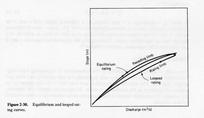
Fig. 2-30
|
|
- Two other mechanisms have a bearing in the evaluation of stage-discharge relations:
- short-term and
- long-term
sedimentation effects.
- Short-term effect: The amount of boundary friction varies with flow rate.
- During low flow, the bed friction consists of grain and form friction.
- During high flows, form friction is eliminated, reducing only to grain friction.
- The reduced friction gives rivers the capability to carry a greater discharge for a given stage
(See Kennedy: Reflections on rivers).
- This explains the shift from low-flow rating to high-flow rating.
- Long-term sedimentation effect: Rivers continuously subject their boundaries to endless cycles of erosion and deposition,
depending on the sediment load they carry.
- Shifts in rating curve are the net result of these natural geomorphic processes.
Rating curve formulas
- In spite of complexities, rating curves are a useful and practical tool in hydrologic analysis, allowing the direct conversion of stage to
discharge and viceversa.
- A widely used rating curve model is the following:
- The proper value of reference stage ho
is that which makes the stage-discharge data plot as close as possible to a straight line on log paper.
- Subsequently, values of constants a and b are determined by regression analysis.
Streamflow variability
- Streamflow varies seasonally, annually, and with geographic location.
- On a global basis, total runoff volume is about 30% of the total precipitation volume.
- The rest is accounted for by evaporation and evapotranspiration.
- The runoff coefficient could be as low as 2% (Arizona) and as high as 93%
(one special case in the Phillipines).
Seasonal variability
- In humid climates, seasonal variability is not marked.
- The Amazon river has a ratio of high-to-low flow of about 3-5.
- In arid climates, seasonal variability is very marked.
- Streams in arid climates may have a ratio of high-to-low flow of 1000 or more.
- For ephemeral streams, this ratio is ∞ (infinity).
- In humid climates, there is contributions of indirect runoff (groundwater flow) throughout the year.
- In arid climates, the water table lies deep in the soil profile, and the contribution of groundwater to surface water is absent.
- Groundwater reservoirs serve as the mechanism for the storage of large amounts of water, which are slowly transported to lower elevations.
- The process is slow and subject to a substantial amount of diffusion.
- The net effect is that of a permanent contribution to surface flow in the form of baseflow.
Annual variability
- Annual streamflow variability is linked to the relative contributions of direct and indirect runoff.
- During dry years, rainfall goes on to replenish the catchment's soil moisture, with little of it showing as direct runoff.
- During wet years, the catchment's storage capacity fills up quickly, and any additional amount is entirely converted into surface runoff.
- A line of inquiry is to focus on the mechanics of coupled surface and groundwater flow.
- This is a very complex process, spatially distributed and temporally varying.
- We have relied on statistics to compensate for the incomplete knowledge of the physical processes.
- This has led to the concept of flood frequency.
- A flood series is extracted from the stream gaging data.
- The statistical analysis of the flood series allows the calculation of flow rates associated with selected frequencies or return periods.
- The procedure is limited by the record length, i.e., the number of years of data.
- With 10 years of data, do not expect to get an accurate value of the 100-yr flood.
Daily flow analysis
- Variability of streamflow can be expressed in terms of the day-to-day fluctuation of flow rates at a given station.
- Differences are due to the climate and the nature of catchment response.
- Small and midsize catchments will usually have steep gradients and concentrate flows with negligible runoff diffusion,
producing hydrographs with many high peaks and low valleys.
- Large catchments are likely to have milder gradients and therefore, to concentrate flows with substantial runoff diffusion.
- The diffusion mechanism acts to spread the flow in time and space, smoothing out the peaks and valleys of the hydrographs.
Flow-duration curve
- Daily flow records are obtained for one or more years.
- The length of the record indicates the total number of days in the series.
- The daily flow series is sequenced in decreasing order, from highest to lowest, and an order number assigned.
- For each flow value, the percent time is the ratio of its order number divided by the total number of days,
and multiplied by 100.
- The flow-duration curve is obtained by plotting flow vs percent time.
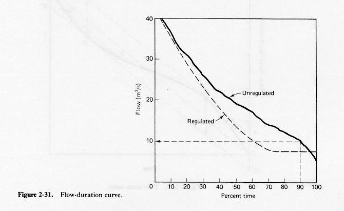
Fig. 2-31
|
|
- The flow-duration curve allows the evaluation of the permanence of characteristic low-flow levels.
- For instance, the flow expected to be exceeded 90% of the time can be readily determined from a flow-duration curve.
- The permanence of low flows is increased with streamflow regulation.
- The usual aim is to assure the permanence of a certain low-flow level 100% of the time.
- Regulation causes a shift in the flow-duration curve by increasing the permanence of low flows while decreasing that of high flows.
- Flow-mass curve.
Geographical variability of streamflow
- Two variables help describe the geographical variability of streamflow:
- catchment area,
- mean annual precipitation.
- The volume available for runoff is directly proportional to the catchment area.
- This is limited by the available precipitation.
- Catchment area is important because large catchments have milder overall gradients.
- This causes increased runoff diffusion, increasing the chances for infiltration.
- The net effect is a decrease of peak discharge per unit area.
- Peak flows are directly related to catchment area (Eq. 2-52).
- The exponent n is generally less than 1, because of runoff diffusion.
- Therefore, peak flow per unit of catchment area is:
- where m = 1 - n.
- This equation confirms that qp is inversely related to drainage area.
- The Creager curves (Fig. 2-33) is an early example of this trend.
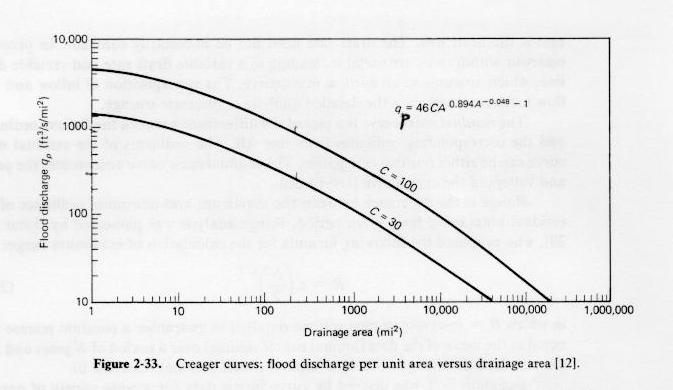
Fig. 2-33
|
|
- Values of C in the range 30-100 encompass most of the data compiled by Creager in the 1930's.
- This range can be taken as a measure of the regional variability of flood discharges.
- However, there is no connotation of frequency to the calculated results.
Go to
Chapter 3.
|