- At equilibrium state, the outflow must equal the inflow. Therefore:
in which:
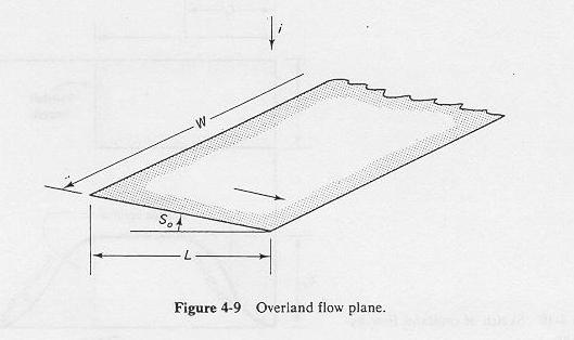
- qe= equilibrium outflow in L/s/m
- i = rainfall excess in mm/hr
- L = plane length in m.
- This equation is a statement of runoff concentration.
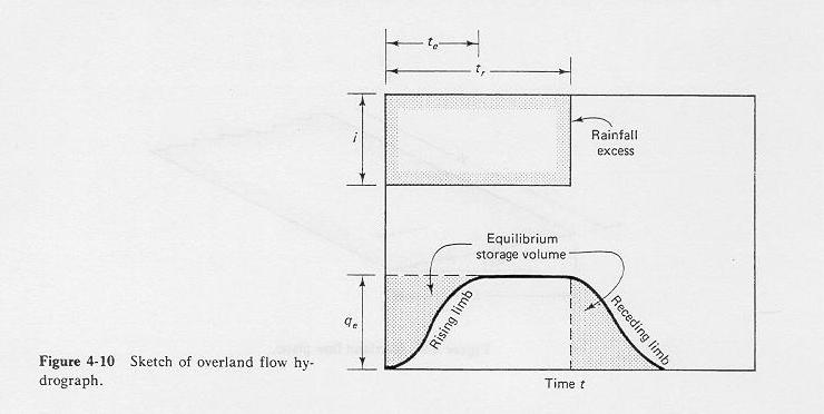
- The equilibrium storage volume is the area above the rising limb and below a line q = qe.
- As a first approximation, it can be assumed to be equal to:
[Eq. 4-20]
in which:
- Se= equilibrium storage volume in L/m
- qe= equilibrium outflow in L/s/m
- te = time to equilibrium in seconds.
- Irregularities cause the equilibrium state to be approached asymptotically, and the actual time to equilibrium is not clearly defined.
- A value of t corresponding to q = 0.98 qe may be taken as an approximation.
- Equations of continuity and motion: Equations 4-21 and 4-22.
- Solutions can be attempted with:
- Storage concept of Horton and Izzard (conceptual) (1940's)
- Kinematic wave technique of Wooding (deterministic) (1960's)
- Diffusion wave technique (1990's) (Ponce, 1986;
HEC-1, 1990;
HEC-HMS, 1998)
- Dynamic wave technique (Ben-Zvi) (1970's).
Overland flow solution based on storage concept
- Horton noticed that experimental data justified a relationship between equilibrium outflow and equilibrium storage as follows:
[Eq. 4-23]
in which a and m are empirical constants.
- A mean flow depth is defined as follows:
[Eq. 4-24]
- Combination of these equations leads to:
[Eq. 4-25]
- in which b = a Lm, another constant.
- Typical values of the rating exponent m are shown in the following table.

Table 4-3
|
|
- From the previous equations 4-20 and 4-23, an estimate of time to equilibrium is:
|
te = 2 / { qe[(m-1)/m] a(1/m) }
|
- For laminar flow conditions, b = a Lm = CL, where CL is
[Chow, Chapter 6]
- The time to equilibrium under laminar flow is:
|
te = (2 L 1/3) / [ i2/3 CL1/3 ]
|
- For turbulent flow conditions, b = a Lm = (1/n) So1/2.
- The time to equilibrium under mixed laminar-turbulent and fully turbulent conditions is:
|
te = 2 (nL)1/m / { i(m-1)/m So[1/(2m)] }
|
To derive the preceding equation, combine the following equations:
|
Se = (qe te)/2
(Horton's assumption for equilibrium storage)
|
|
he = Se / L
(equilibrium flow depth based on equilibrium storage)
|
|
qe = (1/n) So1/2 hem
(turbulent Manning flow rating)
|
- Notice that time to equilibrium increases with friction and plane length, and decreases with rainfall intensity and plane slope.
- This is the same form as Papadakis and Kazan's 1987 formula for time of concentration.
- The friction parameter is similar to Manning's, but can accomodate mixed laminar-turbulent flow.
- For that purpose, it is also referred to as N.
- Typical values of N are shown in the following table.
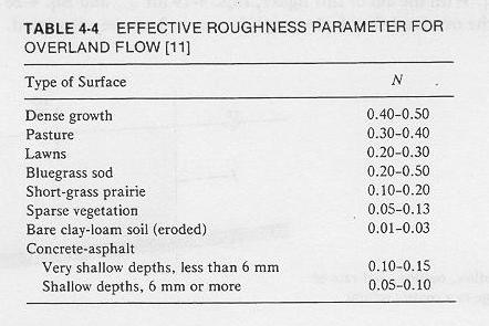
Table 4-4
|
|
- The Horton-Izzard solution is based on the assumption that the discharge-storage rating is valid not only at equilibrium but also at any other time.
- This assumption is convenient because it allows an analytical solution for the shape of the overland flow hydrograph.
- The generic discharge-storage equation represents a nonlinear reservoir, replacing the equation of motion.
- Horton's overland flow model is shown in page 140.
- Horton's solution is for m = 2 (mixed laminar-turbulent flow); Izzard's is for m = 3 (laminar flow).
- The graphical form of Izzard's overland flow model is shown in page 141.
Overland flow solution based on kinematic wave theory
- According to this theory, the equation of motion can be approximated by a depth-discharge rating of the form:
- in which b and m are empirical constants.
- Unlike Horton's approach, which is based on reach volume data,
the kinematic wave approach bases the rating on cross-sectional data such as flow depth.
- The Horton approach is lumped; the kinematic wave approach is distributed.
- The difference between a rating based on storage vs one based on flow depth merits careful analysis.
- There are two distinct features in natural catchments:
- reservoirs, and
- channels.
- In an ideal reservoir, the water surface slope is zero, and therefore, outflow and storage are uniquely related.
- Outflow can be uniquely related to storage volume, stage and flow depth.
- In an ideal channel, the water surface slope is nonzero, and storage is a nonunique function of both inflow and outflow.
- At any cross section, discharge can only be related to flow depth.
- In the Horton approach (reservoir), outflow is related to storage, and by extension, to the mean flow depth on the overland flow plane.
- In the kinematic approach (channel), outflow is related to its flow depth.
- The typical overland flow problem has a nonzero water surface slope; it should behave more as a channel that a reservoir.
- It would appear that the kinematic approach is better suited since it simulates channels bettter than reservoirs.
- However, the kinematic approach lacks runoff diffusion, while there is diffusion in the storage concept.
- When diffusion is at issue, the storage concept is better than the kinematic wave.
- The kinematic wave assumption amounts to substituting a uniform flow formula for the equation of motion.
- It says that, as far as momentum is concerned, the flow is steady!
- However, the unsteadiness is preserved through the continuity equation.
- The implication of kinematic flow is that unsteady flow can be visualized as a sucession of uniform flows, with the water surface slope remaining
constant at all times.
- This can be reconciled with reality only if the changes in stage occur very gradually.
- The changes in momentum should be negligible compared to the forces driving the steady flow (gravity and friction).
- The kinematic flow number of Woolhiser and Liggett determines whether a flow can be considered kinematic or not.
- The kinematic wave model is shown in
page 143 and
page 144.
- The time to equilibrium of kinematic flow is:
|
tk = (nL)1/m / { i(m-1)/m So[1/(2m)] }
|
- This is the same as Horton's mixed laminar-turbulent equation, but without the factor 2.
- The analytical solution to the kinematic wave, a deterministic model, is a parabola, with no diffusion.
- The analytical solution to Horton's conceptual model is a hyperbolic tangent.
- See graphical comparison of dimensionless
overland flow hydrographs.
- Very important: Lack of diffusion means that the kinematic wave is about twice as fast as the storage concept solution.
- Woolhiser and Liggett's kinematic flow number is:
- in which F = Froude number.
- Values of K greater than 20 describe kinematic flow.
- The steeper the slope, the greater the K value, and the more kinematic the flow is.
- Other variables in definition of kinematic flow number are secondary.
- The kinematic wave solution accounts for only friction slope and plane slope.
- For very mild plane slopes, the neglected terms (pressure gradient and inertia) may be promoted to the point
where neglect is no longer justified.
- Most overland flow have steep slopes, usually greater than 0.01.
- Rule of thumb: any slope greater than 0.01 (1 percent) is kinematic.
- For slopes of about 0.0001, the kinematic wave may not be sufficient.
- The kinematic wave celerity varies with the flow, making the kinematic wave a nonlinear equation.
- This property leads to a steepening tendency (inbank flows).
- Flood waves do not steepen
- Analytical solutions, if carried long enough, lead to the
kinematic shock, due to the steepening of the kinematic wave.
- In nature, small irregularities produce diffusion, which arrests the steepening.
- Numerical solutions have numerical diffusion, which also arrests the steepening.
- If the solution is perfect, with no irregularities or errors, it will eventually develop into a shock.
- Due to natural irregularities, kinematic shock may be a rare occurrence in nature.
Overland flow solution based on diffusion wave theory
- According to diffusion theory, the flow depth gradient is largely responsible for the diffusion mechanism.
- Its inclusion in the analysis provides runoff concentration with diffusion.
- Diffusion wave equations: page 146 and
page 147.
- The hydraulic diffusivity is:
- in which u, h, and S are mean velocity, flow depth and channel slope, respectively.
- For very small values of slope, channel diffusivity is very large.
- For zero slope (horizontal channel), the equations ceases to apply.
- For realistic slopes in the range 0.001-0.0001 the diffusion component can be quite significant.
- Diffusion waves apply for the milder slopes for which the kinematic wave is not applicable.
Summary
- Overland flow can provide more detail than the rational method.
- This increased detail is at a cost of increased complexity.
- Overland flow is suited for computer applications.
- However, the problem of conversion of rainfall to runoff is not just one of overland flow.
- It also includes the abstraction from total rainfall to effective rainfall (see Runoff curve number method in Chapter 5).
Go to
Chapter 5A.
|