CIVE 445 - ENGINEERING HYDROLOGY

CHAPTER 5C: HYDROLOGY OF MIDSIZE CATCHMENTS, TR-55 METHOD

5.3  TR-55 METHOD

  • TR-55 is a collection of simplified procedures developed by the NRCS (ex SCS).

  • It consists of two main procedures:

    1. graphical,

    2. tabular.

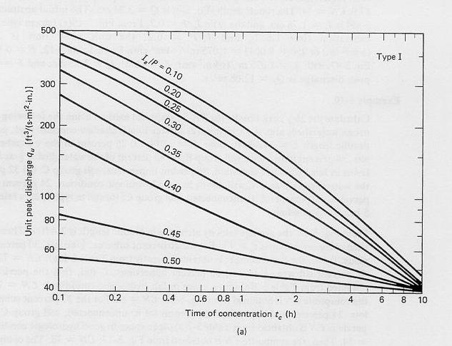
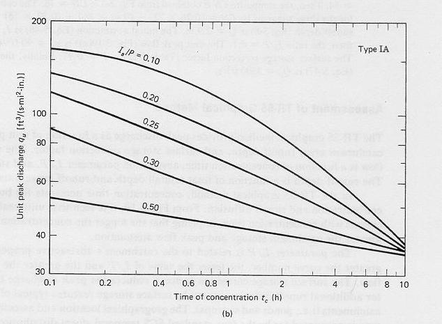
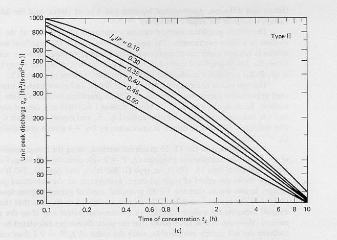
  • The graphical method calculates peak flows, for catchments with time of concentration in the range 0.1-10 hr.

  • The tabular method calculates flood hydrographs, for catchments with time of concentration in the range 0.1-2 hr.

  • The graphical method is described here.
 

TR-55 storm, catchment, and runoff parameters

  • Rainfall in TR-55 is described in terms of total rainfall depth and one of four type rainfall distributions: I, IA, II, and III.

  • These type distributions are shown in Page 189.

  • The location for these type distributions is shown in Page 190.

  • The duration is 24 hr.

  • This constant duration was selected because most rainfall data is reported on a 24-hr basis.

  • Rainfall intensities corresponding to durations shorter than 24 hr are contained within the SCS distributions.

  • For instance, if a 10-yr 24-hr rainfall is used, the 1-hr period with the most intense rainfall corresponds to the 10-yr 1-hr rainfall depth.

  • TR-55 uses the CN method to abstract total rainfall.

  • TR-55 is intended to be used for midsize basins, greater than 2.5 km2, with time of concentration up to 10 hours.

  • Therefore, TR-55 includes procedures to determine the time of concentration for the following three types of surface flow:

    1. overland flow,

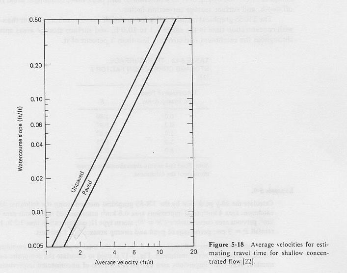
    2. shallow concentrated flow, and

    3. channel flow.


Selection of runoff curve number CN

  • TR-55 defines two types of areas in urban catchments:

    1. pervious

    2. impervious

  • Runoff curve numbers are calculated by areal weighing.

  • Impervious areas are of two types:

    1. connected

    2. unconnected

  • Connected impervious areas are those in which runoff flows directly into the drainage system, or where runoff (from the impervious area) flows over a pervious area as shallow concentrated flow (as in a grass-lined swale).

  • Unconnected impervious areas are those in which runoff (from the impervious area) flows over a pervious area (as overland flow) before it enters the drainage system.  


  • Table 5-2(a) shows urban runoff curve numbers for different classes of pervious areas and connected impervious areas.

  • Table 5-2(b), Table 5-2(c), and Table 5-2(d) show runoff curve numbers for agricultural lands, forest, and semiarid rangelands, respectively.

  • Figure 5-16 is used in lieu of Table 5-2 if the impervious area percentages or the pervious area classes are other than those shown in the table (table shows only typical values).

  • When the impervious areas are unconnected, Fig. 5-16 is used in cases where the total impervious area exceeds 30% of the catchment.

  • Fig. 5-16 gives a composite CN as a function of percent imperviousness and pervious area CN.

  • Figure 5-17 is used to determine the composite CN when all or portions of the impervious areas are unconnected and the total impervious area is less than 30%.

  • Fig. 5-17 gives a composite CN as a function of percent imperviousness, ratio of unconnected impervious area to total impervious area, and pervious area CN.
 

Travel time and time of concentration

  • For any reach or subreach, travel time is defined as the ratio of flow length to average flow velocity.

  • At any given point in the catchment, the time of concentration is the sum of travel times through the upstream reaches.

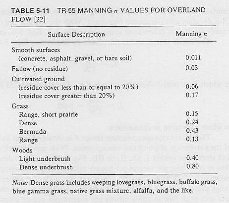
  • For overland flow, TR-55 uses the following formula for travel time:

    tt = [0.007 (nL) 0.8] / [P2 0.5 S 0.4]

    in which tt = travel time in hours, n = Manning's n, L = flow length in ft, P2 = 2-yr 24-hr rainfall in inches, and S = average land slope, in ft/ft.

  • In SI units, the travel time is:

    tt = [0.0288 (nL) 0.8] / [P2 0.5 S 0.4]

    in which L = flow length in m, P2 = 2-yr 24-hr rainfall in cm, and S = average land slope, in m/m.

  • Table 5-11 shows values of Manning's n applicable to overland flow.

  • Overland flow lengths more than 300 ft lead to a form of surface flow referred to as shallow concentrated flow.

  • For shallow concentrated flow, the average flow velocity is determined from Figure 5-18.


TR-55 graphical method

  • The TR-55 graphical method calculates peak discharge based on the concept of unit peak flow.

  • The unit peak flow is the peak flow per unit area per unit runoff depth.

  • Unit peak flow is a function of

    1. time of concentration,

    2. ratio of initial abstraction to total rainfall, and

    3. storm type.

  • Peak discharge is calculated by the following formula:

    Qp = qu A Q F

    in which:

    • Qp = peak discharge (L3T-1)

    • qu = unit peak flow (T-1)

    • A = area, (L2)

    • Q = runoff depth (L)

    • F = surface storage correction factor (dimensionless).

  • It is first necessary to evaluate the catchment flow type (overland flow, shallow concentrated flow, or channel flow).

  • The time time of concentration is evaluated with formulas or graphs.

  • The runoff curve number CN is determined from tables or figures.

  • A flood frequency is selected.

  • The rainfall depth P for the 24-hr duration and chosen frequency is determined from depth-duration-frequency maps.

  • With P and CN, the runoff Q is determined by the curve number method.

  • The initial abstraction Ia is estimated as 20% of the potential maximum retention S (standard value of NRCS initial abstraction):

    Ia = 0.2 S

  • S is mapped to CN by the Mockus mapping equation:

    S = (1000/CN) - 10

  • from which the initial abstraction in inches, is:

    Ia = (200/CN) - 2

  • The initial abstraction in cm, is:

    Ia = (508/CN) - 5.08

  • The surface storage correction factor F is obtained from Table 5-12.

  • With time of concentration tc, initial abstraction ratio Ia/P, and storm type (I, IA, II, or III), the unit peak flow is determined from the TR-55 graphical charts.


    Type I

    Type IA

    Type II

    Type III

  • Interpolation can be used for values of Ia/P other than those shown.

  • For values out or range, the maximum or minimum value shown should be used.

  • To obtain unit peak flow in SI units (m3s-1km-2cm-1), the values of the graphs are multiplied by the conversion factor 0.0043.

  • Peak discharge is calculated by the following formula:

    Qp = qu A Q F

  • TR-55 method is limited to:

    • CN greater than 40,

    • time of concentration between 0.1 and 10 hours, and

    • surface storage areas throughout the catchment and covering at most 5% of it.


Assessment of TR-55 graphical method

  • Time of concentration accounts for both runoff concentration and diffusion.

  • The unit-peak-flow graphs show that unit peak flow decreases with time of concentration.

  • This implies that diffusion increases with catchment size and time of concentration.

  • This is the same finding than Creager's (See Creager curves).

  • The parameter Ia/P is related to the catchment's abstractive properties.

  • The factor F reduces the peak discharge to account for additional runoff diffusion caused by surface storage features typical of low-relief catchments (ponds and swamps).

  • The climate and geographical location is accounted for by the storm type distributions.

  • Thus, the TR-55 method accounts for hydrologic abstraction, runoff concentration and diffusion, climate and geographical location, and depression storage.

  • The TR-55 method is an extension of the rational method to midsize catchments.

  • The unit peak flow qu (peak discharge per unit area per unit runoff depth) is similar to the runoff coefficient C (peak discharge per unit drainage area per unit rainfall intensity).

  • Unlike the rational method, the TR-55 method is applicable to midsize catchments.  


Comparison with the rational method

  • Assume A = 1 mi2, I = 1 in/hr, C = 0.95 (high).

  • A calculation with the rational method gives: Qp = C I A = 613 cfs.

  • A calculation with the TR-55 method, using the lowest possible value of abstraction (Ia/P = 0.10, roughly equivalent to C = 0.95), gives the following results:

    • For storm type I: Qp = 200 cfs.

    • For storm type IA: Qp = 108 cfs.

    • For storm type II: Qp = 360 cfs.

    • For storm type III: Qp = 295 cfs.

  • This example shows the effect of the storm type on the calculated peak discharge by the TR-55 method.

  • The type II storm is the most intense, while the type IA storm is the least intense.

  • This example shows that the TR-55 method gives generally lower values than the rational method.

  • This is to be expected, since the TR-55 method is accounting for runoff diffusion in a better way than the rational method.

  • The graphs were developed by running the TR-20 computer model many times.

  • Conclusion: Use TR-55 method to develop peak discharges for midsize catchments.


Go to Chapter 6.

 
060322