|
|
CIVE 445 - ENGINEERING HYDROLOGY
CHAPTER 8: RESERVOIR ROUTING
|
- In many applications, it is necessary to calculate the variation of flows in time and space.
- These applications include
- reservoir design,
- design of flood-control structures,
- flood forecasting, and
- water resources planning and management.
- Surface-water reservoirs store water for
- hydropower generation,
- municipal and industrial water supply,
- flood control,
- irrigation,
- navigation,
- fish and wildlife management,
- enhancement of water quality, and
- recreation.
- Reservoir routing uses mathematical relations to calculate outflow from a reservoir, once the
following are known:
- inflow,
- initial conditions,
- reservoir characteristics, and
- operational rules.
- The classical approach to reservoir routing is based on the storage concept.
- Hydrologic reservoir routing is based on the storage concept.
- Hydraulic reservoir routing is based on the complete equations of motion.
- Types of reservoirs, depending on type of outflow:
- Uncontrolled: free flowing
- Controlled: with gates
- A combination of controlled and uncontrolled.
- Types of reservoirs with uncontrolled outflow:
- Simulated: uses mathematical relations to simulate natural diffusion processes; the
linear reservoir method.
- Actual: refers to routing through planned or existing reservoir; the
storage indication method.
- Flow through an emergency spillway is usually of the uncontrolled type.
- Catchment routing with linear reservoirs is simulated.
- Reservoir design (geometric features) is accomplished with actual (storage-indication) reservoir routing models.
Storage-Outflow Relations
- In an ideal reservoir, storage is a function of outflow only.
- The general relationship between outflow and storage is:
- A common relationship between outflow and storage is:
- Figure 8-1.
- For n = 1, we get the linear reservoir:
- The linear reservoir equation is applicable to simulated routing.
- The nonlinear reservoir equation is applicable to actual routing.
- Exception: Spillway in Colorado, where a linear reservoir was actually built!
- In linear reservoir routing, the constant K represents the amount of storage or diffusion.
- Greater values of K result in increased outflow hydrograph diffusion.
- For actual reservoirs and spillways, the nonlinear properties of the storage-outflow relations
must be determined in advance.
- Outflow will depend on whether the flow is discharged through either closed conduit(s), overflow spillway(s),
or a combination of the two.
- A general outflow formula is the following:
- Z represents either the cross-sectional area in close conduits, or the length of the crest in an
overflow spillway.
- Cd is the discharge coefficient; H is the hydraulic head; y is the rating exponent.
- Theoretical values of Cd and y are determined using hydraulic principles.
- For the free-outlet closed conduit, the conservation of energy between reservoir pool and outlet elevations,
neglecting entrance and friction losses, leads to:
- Therefore, the outflow is:
- It follows that y = 1/2 and Cd = 4.43 in SI units and 8.02 in U.S. customary units.
- These theoretical values are reduced by about 30% to account for flow contraction and entrance losses.
- For an ungated overflow spillway, the critical flow condition
[flow depth y = (2/3) H] in the vicinity of the crest leads to:
|
O = V A = [g (2/3)H)1/2 [(2/3)H] Z
|
which reduces to:
|
O = (2/3) [(2/3)g] 1/2 Z H 3/2
|
- It follows that y = 3/2 and Cd = 1.7 in SI units and 3.09 in U.S. customary units.
- In practice, the discharge coefficient of an overflow spillway is not constant, varying with H
between 85 and 130% of the theoretical value (that assumes critical flow in the vicinity of the crest).
- In the proportional (or linear reservoir) overflow spillway (weir),
the cross-sectional flow area grows in proportion
to the half-power of H.
- Therefore, outflow is linearly related to H, and a linear storage-outflow rating is applicable.
- Spillway Photos.
|
1.2 LINEAR RESERVOIR ROUTING
|
- The differential equation of storage can be solved by analytical or numerical means.
- The numerical approach is preferred because it can take an arbitrary inflow hydrograph
and can be solved with the computer.
- The solution is accomplished by discretization on the x-t plane.
- The discretization leads to:
|
(I1 + I2) / 2 - (O1 + O2) / 2 = (S2 - S1) / Δt
|
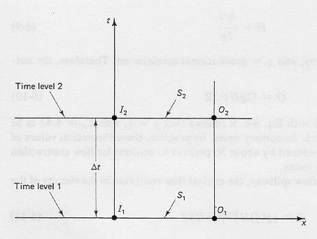
Fig. 8-2
|
- At each time level, the linear reservoir storage-outflow relation is satisfied:
- Substituting these equations into the discretized differential equation of storage:
- in which the routing coefficients are defined as follows:
|
C0 = (Δt/K) / [2 + (Δt/K)]
|
|
C2 = [2 - (Δt/K)] / [2 + (Δt/K)]
|
- Since C0 + C1 + C2 = 1, the routing coefficients are interpreted as
weighting coefficients.
- These coefficients are a function of Δt/K.
- Values of routing coefficients as a function of Δt/K are shown in
Table 8-1.
- Example 8-1.
- Example 8-1 Graph.
- The peak flow is attenuated and the time base increased.
- In the linear reservoir case, the amount of attenuation is a function of Δt/K.
- The smaller this ratio, the greater the amount of attenuation exerted by the reservoir.
- Values of Δt/K greater than 2 can lead to negative outflows; this should be avoided.
- Peak outflow occurs at the time when inflow equals outflow; see
Example 8-1 Graph.
- Since outflow is proportional to storage, peak outflow corresponds to peak (or maximum) storage.
- Peak storage occurs when outflow equals inflow; after this, outflow is drawing from storage.
- Therefore, peak outflow occurs when outflow equals inflow.
- Reservoir routing has an immediate outflow response, see
Example 8-1 Graph.
- There is no lag between the start of inflow and the start of outflow.
- This property is due to the fact that in an ideal reservoir, with water surface slope equal to zero,
surface water have an infinite velocity of propagation.
- In other words, when the Froude number is zero (u = 0), the celerity of surface waves is infinity.
|
1.3 STORAGE-INDICATION METHOD
|
- The storage indication method is used to route flood waves through actual reservoirs.
- The storage indication method is also known as the Modified Puls method.
- The method is based on the discretization of the differential equation of storage.
- Discretization on the x-t plane leads to:
|
(I1 + I2) / 2 - (O1 + O2) / 2 = (S2 - S1) / Δt
|
- Putting all unknowns in the LHS:
|
(2S2/Δt) + O2 = I1 + I2 + (2S1/Δt) - O1
|
- The LHS is known as the storage-indication quantity.
- It is first necessary to assemble geometric and hydraulic reservoir data in suitable form.
- For this purpose, the following curves (or tables) are prepared:
- Elevation-storage: obtained from the geometry (topography and bathymetry) of the reservoir.
- Elevation-outflow: obtained from the hydraulic properties of the spillway (weir or closed-conduit spillway)
- Storage-outflow: obtained from the first two curves (for the same elevation, the corresponding storage
and outflow).
- Storage indication-outflow: obtained from the storage-outflow relation
[for each pair of storage-outflow, create a storage indication (2S/Δt + O) and plot this quantity vs outflow].
- The time interval Δt is selected to linearize the inflow hydrograph.
- It should be at least 1/5 of the time-of-rise of the inflow hydrograph.
- Application of the storage-indication method consists of a recursive procedure:
- Set the counter n = 1 to start.
- Use the discretized storage-indication equation to calculate the storage indication quantity
(2S/Δt + O) at time level n+1:
(2Sn+1/Δt + On+1)
- With (2Sn+1/Δt + On+1),
use the storage-indication vs outflow relation to calculate On+1.
- With (2Sn+1/Δt + On+1) and On+1,
calculate:
(2Sn+1/Δt - On+1).
- Increment the counter by 1, and go back to step 2 and repeat.
- The procedure is illustrated by
Example 8-2 and
Table 8-3.
- The results of Table 8-3 Column 5 are the same as those of Table 8-2 Column 6.
- This confirms that a linear reservoir can be also routed with the storage-indication method.
- The application of the
storage-indication method to an actual reservoir (Turner reservoir, San Diego North County) is
shown by Example 8-3
-
Example 8-3: Table 8-4
-
Example 8-3: Figure 8-4
-
Example 8-3: Table 8-5
|
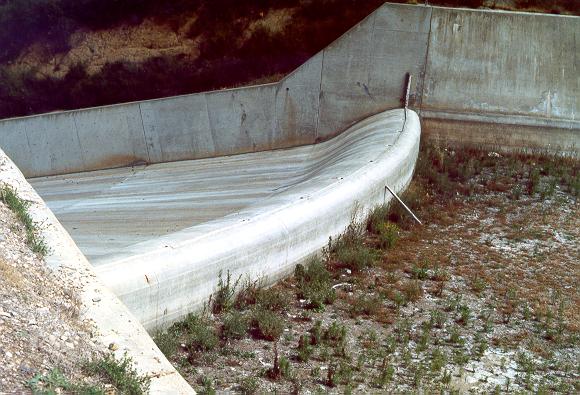
Spillway of Turner reservoir, San Diego County. |
|
Go to
Chapter 9A.
|
