Kinematic wave equation

• The derivation of the kinematic wave equation is based on the principle of mass conservation within a control volume.

• The difference between outflow and inflow within one time interval is balanced by a corresponding change in volume.

• In terms of finite intervals, it is:

  (Q2 - Q1) Δt + (A2 - A1) Δx = 0

• The differential form can be written as:

  ∂Q/∂x + ∂A/∂t = 0

• The equation of conservation of momentum (Eq. 4-22) contains local inertia, convective inertia, pressure gradient, friction, gravity, and a momentum source term.

• The kinematic wave uses a statement of steady uniform flow in lieu of conservation of momentum.

• This simplification limits the applicability of kinematic waves.

• The Manning equation of steady uniform flow is:

  Q = (1/n) A R2/3Sf1/2

• The Chezy equation of steady uniform flow is:

  Q = C A R1/2Sf1/2

• The hydraulic radius R = A/P. Substituting this into the Manning equation leads to:

  Q = (1/n) (Sf1/2/P2/3) A5/3

• Assume that n, S_f and P are constants, for simplicity.

• This is the case of a wide channel with little bed movement.

• This equation can be written as:

  Q = α Aβ

  in which α and β are parameters of the discharge-area rating.

  α = (1/n) Sf1/2/P2/3

  β = 5/3

• Differentiating the discharge-area rating leads to the kinematic wave celerity:

  dQ/dA = αβAβ-1 = β(Q/A) = βV

  in which V = mean flow velocity.

• Multiplying the continuity equation with the kinematic wave celerity equation (chain rule), leads to:

  ∂Q/∂t + (dQ/dA) ∂Q/∂x = 0

  or, alternatively:

  ∂Q/∂t + (βV) ∂Q/∂x = 0

• These two equations describe flood wave movement (unsteady flow) under the kinematic wave assumption.

• Kinematic waves travel with celerity βV.

• The kinematic wave equation is a first-order partial differential equation.

• Therefore, it cannot describe diffusion or attenuation.

• Diffusion is a second-order process.

• Since dQ/dA is the celerity, it can be replaced by dx/dt. Therefore:

  ∂Q/∂t + (dx/dt) ∂Q/∂x = 0

• This is equal to the total derivative dQ/dt.

  dQ = (∂Q/∂t) dt + (∂Q/∂x) dx = 0

• Since RHS = 0, it follows that Q remains constant in time for waves traveling with celerity dQ/dA.

Discretization of kinematic wave equation

• The kinematic wave equation is nonlinear and of first-order.

• It is nonlinear because the wave celerity varies with discharge.

• The nonlinearity is usually mild, and for some applications, the equation can be considered to be linear.

• The solution can be obtained by analytical or numerical means.

• The simplest kinematic wave solution is a linear numerical solution.

• It is necessary to select a numerical scheme and its properties.

Order of accuracy of numerical schemes

• The order of accuracy of a numerical scheme measures the ability of the numerical scheme to reproduce the terms of the differential equation being solved.

• In general, the higher the order, the better the reproduction of the differential equation.

• Forward and backward finite-difference schemes have first-order accuracy.

• Central schemes have second-order accuracy.

• First-order schemes create numerical diffusion and dispersion.

• Second-order schemes create only numerical dispersion.

• A third-order scheme of the kinematic wave equation creates neither numerical diffusion or dispersion.

• A third-order scheme reproduces exactly the terms of the differential equation.  

   

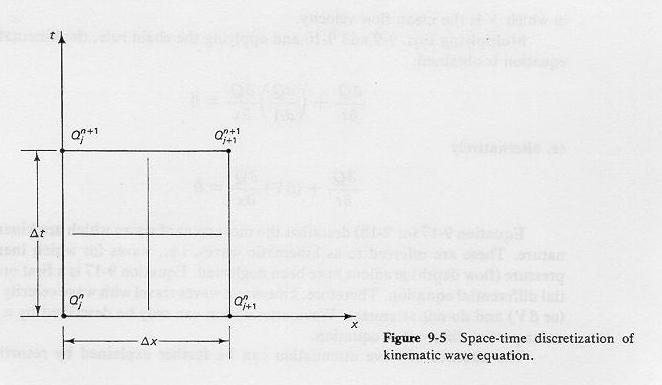
  Fig. 9-5

   

• Second-order accurate numerical scheme, central differences in time and space: Example 9-3.

• Second-order accurate numerical scheme: Example 9-3 (continued)

• The Courant number is defined as the ratio of wave celerity βV to the "grid" celerity Δx/Δt:

  C = βV / (Δx / Δt) = βV (Δt / Δx)

   

• This example illustrates the properties of kinematic waves:
  
  
  • For C =1, there is no numerical diffusion or dispersion; the solution is a kinematic wave, translated by not diffused.

  • For C= 1.5, there is numerical diffusion and dispersion. The diffusion results in slight attenuation; the dispersion causes negative outflows in the tail of the calculated hydrograph.

• The second-order accurate method is impractical because it may lead to negative outflows.  

   

• First-order accurate numerical scheme, backward in time, backward in space: Example 9-4.

• Example 9-4 (continued)

• It is observed that offcentering the derivatives has caused a significant amount of numerical diffusion, with peak outflow 120.93 m³/sec.

• Different schemes will lead to different answers, depending on the Courant number.

Convex method

• The convex method of channel routing belongs to the family of linear kinematic wave methods.

• Until 1982, it was part of the NRCS (ex SCS) TR-20 hydrologic model.

• The routing equation for the convex method is obtained by discretizing the kinematic wave equation in a linear mode with forward differences in time and backward differences in space.

• Convex method, forward in time, backward in space: Convex method.

• Convex method (continued)

• Example 9-5 (continued)

• The convex method is relatively simple, but the answer is dependent on the routing parameter C.

• This can be interpreted as a Courant number.

• However, for values of C other than 1, the amount of numerical diffusion is unrelated to the physical diffusion.

• The convex method is a crude approach to stream channel routing.

Kinematic wave celerity

• The kinematic wave celerity is dQ/dA or βV.

• A value β= 5/3 is applicable to a wide channel with Manning friction.

• In 1900, Seddon concluded that the celerity of long disturbances (read kinematic and diffusion waves) was equal to dQ/dA.

• Since dA= T dy, where T is the channel top width, the Seddon law is expressed in practice as:

  c = (1/T) (dQ/dy)

• with c = kinematic wave celerity.

• The kinematic wave celerity is a function of the slope of the discharge-stage rating and the channel top width.

• Since both dQ/dy and T vary with stage, c varies with the stage.

• If c = βV is a function of Q, then the kinematic wave equation is nonlinear.

• Nonlinear solutions account for the variation of c with stage and flow level.

• Linear solutions assume a constant value of c.

• Note that there is a striking similarity between linear kinematic wave solutions and the Muskingum method.  

• Theoretical β values other than 5/3 can be obtained for other friction formulations and cross-sectional shapes.

• For laminar flow, β = 3.

• For a wide channel with Chezy friction, β = 3/2.

• Calculation of β as a function of frictional type and cross-sectional shape: Example 9-6

• Example 9-6 (continued)

Kinematic waves with lateral inflow

• Practical application of stream channel routing often require the specification of lateral inflows.

• The lateral inflow could be concentrated (tributary flow), or distributed along the channel (groundwater exfiltration or infiltration).

• A mass balance leads to:

  (∂Q/∂x) + (∂A/∂t) = qL

• Multiplying this equation by dQ/dA (or βV) leads to:

  (∂Q/∂t) + (βV) (∂Q/∂x) = (βV) qL

Applicability of kinematic waves

• The kinematic wave is a fundamental streamflow property.

• Flood waves which approximate kinematic waves travel with celerity βV and are subject to negligible attenuation (diffusion).

• In practice, flood waves are kinematic if they are of long duration or travel on a channel of steep slope.

• Usually, slopes greater than 1% are kinematic.

• Criteria for the applicability of kinematic waves to overland flow (Chapter 4, page 145) and stream channel flow has been developed.

• The stream channel criterion is:

  (tr So Vo) / do > N

• where t_r= time-of-rise of the inflow hydrograph; S_o = bottom slope, V_o = average velocity, and d_o = average flow depth.

• For 95 percent accuracy in one period of translation, a value of N = 85 is recommended.

• Example 9-7

Go to Chapter 9C.