CIVE 633 - ENVIRONMENTAL HYDROLOGY
EUTROPHICATION MODELS

Click -here- for printable copy.

GENERAL TYPES OF MODELS

Models for understanding and controlling eutrophication can be classified as:

Watershed models
Waterbody models
Management models

Watershed models provide estimates of nutrient loads reaching a lake or reservoir.
Static models are often used to estimate the annual nutrient (phosphorous) load.
Simulation (dynamic) models require lots of data.
Eutrophication waterbody models range from simple empirical models to more detailed ecological models.
These models are all based on mass balance considerations.
Management models are used to determine the optimal control strategy.

WATERSHED MODELS

A watershed model can provide information on the nutrient sources to a waterbody.
They are particularly useful for estimating non-point source nutrient input.
A watershed model that predicts the average annual total phosphorous inputs from point and non-point sources is often sufficient.
More complex models distinguish between biologically available and unavailable nutrients, and seasonal variations.
Non-point source nutrients are contained in surface runoff and baseflow.
The nutrient content of surface runoff depends on processes on the soil surface.
The nutrient content in baseflow depends on processes on the soil profile.
Empirical watershed models
The simplest models are empirical, of the following form:

A = a_o + a₁X₁ + a₂X₂ + ... + a_mX_m

B = b_o + b₁Y₁ + b₂Y₂ + ... + b_mY_m

in which
A = average annual nutrient load to a waterbody (kg/yr);
X_i = area (ha) of watershed with land use i;
B = average nutrient concentration in streamflow (mg/L);
Y_i = fraction of watershed occupied by land use i;
a = coefficient (kg/ha/yr)
b = coefficient (mg/L)

The values of the coefficients are inferred from water quality sampling data.
Coefficients are "nutrient export coefficients".
Identify a single land-use catchment, and measure the total nutrient flux for several years.
Divide total flux by the number of years and catment area to produce the coefficient (kg/ha/yr).
Extrapolation of empirical formulas is not justified.
Simulation watershed models
These models simulate the physical and biochemical processes which can affect the nutrient sources.
These models describe mathematically the water and nutrient fluxes.
Simple models usually consider a 1-day time interval.

D_kt = d_kt Q_kt TD_kt

S_kt = s_kt X_kt TS_kt

in which
D_kt = dissolved nutrient loss (kg) in runoff or baseflow from area k during time period t;
S_kt = solid-phase (suspended) nutrient loss (kg) in runoff or baseflow from area k during time period t;
Q_kt = runoff or baseflow (m³);
d_kt = dissolved nutrient concentration in runoff or baseflow (kg/m³);
s_kt = solid-phase nutrient concentration in sediment (kg/ton);
X_kt = sediment loss (ton);
TD_kt = fraction of dissolved nutrients which reaches a waterbody from area k (assumed equal to 1 for lack of data); and
TS_kt = fraction of solid-phase nutrients which reaches a waterbody from area k (sediment delivery ratio).

WATERBODY MODELS

Selection of most appropriate model should begin with careful consideration of specific eutrophication control objectives.
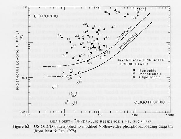
Models predicts total P concentration as a function of the annual P loading.
Errors of simple empirical models can be 30% or more.
Assessment of trophic state can be done with a simple empirical model.
Plots of areal water loading vs phosphorous loading as shown in the figure below.

Another equation is the following:

TP = (L_p/q_s) [1 + (t_w)^0.5]

in which
TP = average annual in-lake total P concentration (micrograms/L);
L_p = annual areal P loading (mg/m²/yr);
q_s = annual areal water loading (m/yr) = z/t_w;
t_w = hydraulic residence time (yr);
z = mean depth (m).

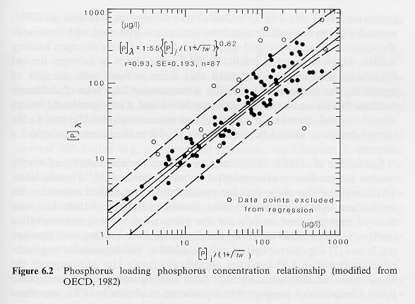
An updated equation is the following:

[P]_λ = 1.55 {[P]_j / (1 + t_w^0.5)} ^0.82

in which
P_λ = average annual in-lake total P concentration (micrograms/L);
P_j = average annual inflow total P concentration (micrograms/L) (= L_p/q_s);

Simulation waterbody models
Mathematical description of the important physical, chemical, and biological processes in lake or reservoir systems.
Dynamic eutrophication models typically contain three types of terms:

Hydrologic and hydrodynamic characteristics
Chemical and biological transformations.
Input, output, or exchange of materials through the boundaries.

Hydrological throughflow determines the flushing rate of a reservoir.
This could be a significant loss factor for algal biomass and nutrients.
Two layers, epilimnion and hypolimnion, are usually considered.
Two- or three-dimensional hydrodynamic models can be very complex.
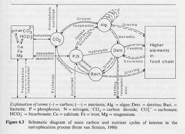
Chemical and biological transformations form core of eutrophication model.
Most eutrophication models concentrate on the biological cycle, rather than on the chemical components.

041117