Simplified

Muskingum Routing Equation


Victor M. Ponce


Online version 2016
[Original version 1979]


 1.  INTRODUCTION

The Muskingum method and its variations are well established in the flood routing literature. Traditionally, its parameters K and X have been determined by calibration using measured inflow and outflow hydrographs. An improved version is due to Cunge (4), who showed that parameters K and X could be related to the physical problem, thus eliminating the need for trial and error calibration while at the same time enhancing the predictive capabilities of the method.

With the aid of Cunge's findings, the calculations can proceed either in a lumped parameter mode (5), or in a variable parameter mode (6,7). The lumped parameter mode has simplicity as its major advantage, although this is achieved at the cost of a certain loss in detail. On the other hand, the variable parameter mode gives up simplicity in return for a greater detail in the definition of the hydrograph. Given the tradeoffs involved, it seems certain that both approaches will continue to be used in the future. Where simplicity is at stake, the lumped parameter model applies; where the need is for greater accuracy, the variable parameter mode is the logical choice.

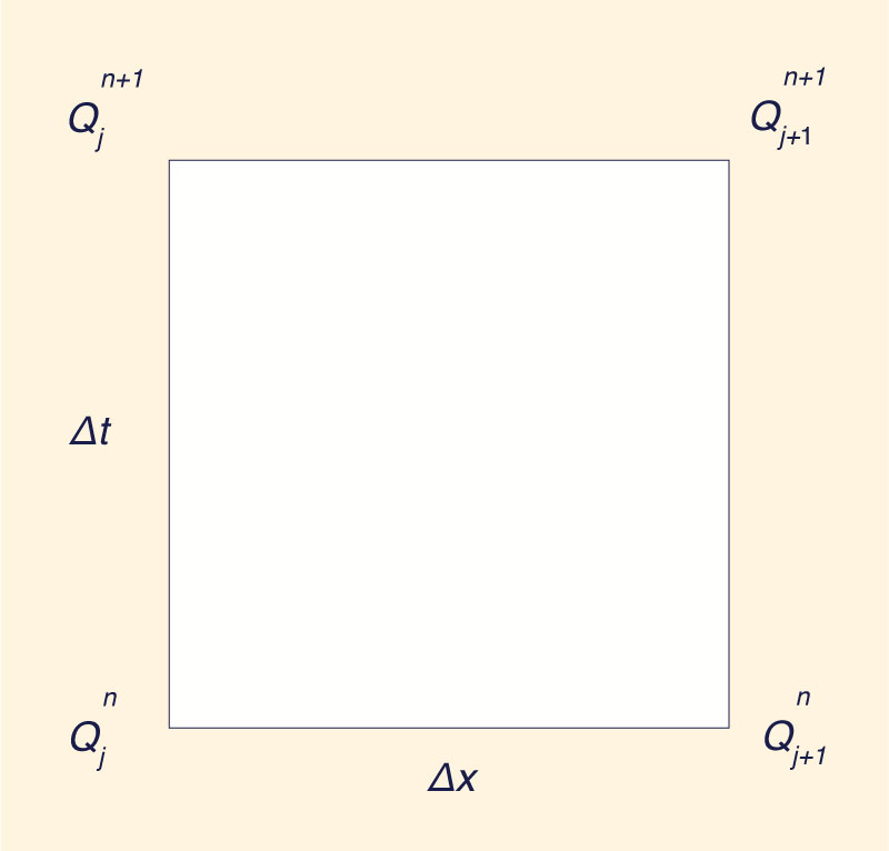
The calculations for the lumped parameter mode can proceed in one of two ways. The conventional way is to specify space and time intervals Δx and Δt; parameters K and X are calculated therefrom. An alternate way is to specify K and X and to calculate Δx and Δt from them. As it will be shown here, the proper choice of parameters can lead to a considerable simplification in the routing equation. This enables the engineer to obtain a reasonably accurate. solution to the flood routing problem with a minimum of computational effort.


 2.  MUSKINGUM METHOD

In the Muskingum method, outflow discharge Qj+1n+1 is expressed as follows (refer to Fig. 1)


Qj+1n+1 = C1 Qj n + C2 Q j n + 1 + C3 Qj + 1 n

(1)

in which C1, C2 and C3 are coefficients defined as follows:

                   Δt
                ______  +  2X
                   K
C1_______________________
              Δt
           ______  +  2 ( 1 - X )
              K
(2)

                  Δt
                ______  -  2X
                   K
C2_______________________
               Δt
            ______  +  2 ( 1 - X )
               K
(3)

                                 Δt
             2 ( 1 - X ) - ______
                                  K
C3_______________________
              Δt
            ______  +  2 ( 1 - X )
               K
(4)


 3.  SIMPLIFIED MUSKINGUM ROUTING EQUATION

In Eqs. 2-4, if Δt /K and X are specified as follows:

     Δt           
   _____  =  1
      K     
(5)

   and X  =  0 (6)

it follows that:

                            1
C1 = C2 = C3 = ______
                            3
(7)

leading to the simplified form of the Musking routing equation as follows:

                   Q j n + Q j n+1 + Q j+1 n            
Qj+1n+1  =  ________________________
                                   3      
(8)

The satisfaction of Eqs. 5 and 6 implies that Δx and Δt are fixed. In effect, K is defined as the time it takes a flood discharge to travel distance Δx with celerity c:

Dimensionless relative wave celerity vs dimensionless wavenumber in unsteady open-channel flow

Fig. 1  Space-time discretization in the Muskingum method.

            Δt           
K  =  ______
            c     
(9)

Therefore, from Eqs. 5 and 9:

            c Δt           
C  =  ________  = 1
             Δx     
(10)

in which C = the Courant number. Equation 10 specifies that the flood wave celerity c be equal to the "grid celerity" Δxt.

Cunge (4) has shown that parameter X can be related to the physical problem as follows:

         1                   q
X  =  ___  ( 1 -  __________ )
         2              So c Δx
(11)

in which q = unit-width discharge; and So = channel bed slope. Equations 6 and 11 lead to:

               q
D  =  __________ = 1
          So c Δx
(12)

in which D = grid Reynolds number. Equation 12 specifies that channel diffusivity q /(2So) be equal to "grid diffusivity" (cΔx)/2. Equations 10 and 12 enable the calculation of Δx and Δt as a function of the flow variables. In this regard, it should be noted that the space interval computed from Eq. 12 is the same as the "characteristic length" on which the Kalinin-Milyukov method is based (6). While this similarity is recognized, the method proposed herein stands on its own merits since it leads to a routing equation (Eq. 8) which is much simpler than that of the Kalinin-Milyukov method.


 4.  CALCULATION OF SPACE AND TIME INTERVALS

From Eqs. 10 and 12, the space and time intervals are given by:


               q           
Δx  =  _______
            So c     

(13)

and


            Δx           q
Δt  =  _____ = ________ 
             c         So c 2

(14)

For natural (nonprismatic) channels, the channel friction and cross-sectional shape are implicitly stated in the steady-state discharge-area relation:


Q = α A β

(15)

in which A = cross-sectional flow area; and α and β = coefficient and exponent, respectively. The flood wave celerity is the kinematic wave celerity defined as follows:


           dQ                              βQ          β B q
c  =  _______ = α β A  β-1  =  _____  =  ________
           dA                                A              A

(16)

in which B = top width. From Eqs. 13 and 16:

                  A           
Δx  =  __________
              β B So     
(17)

and

            Δx               A 2 - β
Δt  =  ______  =  _____________
             c             α β 2 B So     
(18)

As with all lumped parameter models (5), some judgement is required in the choice of the reference hydraulic variables (i.e., q, A and B in Eqs. 16-18) on which to base the calculations of Δx and Δt. The use of average quantities is usually sufficient from the standpoint of accuracy.


5.  MODEL TESTING

The testing of a mathematical model usually hinges upon whether the model can reproduce measured field data. When discrepancies occur, however, it is very difficult and sometimes impossible to determine whether they are due to errors in the numerical solution, in the estimation of the parameters, or in the measured data. A procedure currently open to question (2) consists of lumping all these errors into one, and adjusting the model parameters to fit the measured data in what has been referred to as "calibration".

A sounder approach consists of isolating the sources of error in order to study their effects separately. This is done by performing both a hypothetical test and a real data test. The hypothetical test is designed to isolate the effects of numerical accuracy on the model results. On the other hand, the real data test is designed to provide information on the accuracy of the parameter estimation. Errors in the measured data can only be assessed from a qualitative standpoint.

Hypothetical Test. A hypothetical test using the classical example of Thomas (10) was set up to test the method proposed herein. The following two runs were made: (1) A test run using the simplified method; and (2) a control run using the conventional method. In the test run, X was made equal to zero and K equal to Δt. Accordingly, the space and time intervals were calculated to be Δx = 13.5 miles (21.7 km) and Δt = 2.16 hr.

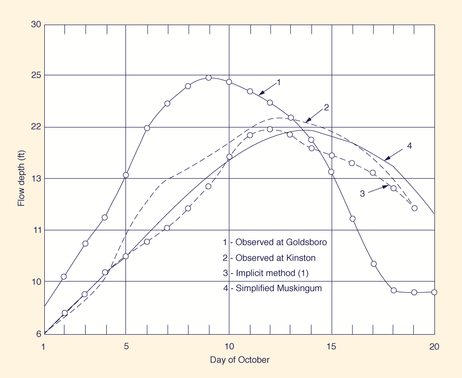
In the control run, the space and time intervals were specified to be Δx = 25 miles (40 km) and Δt = 6 hr. This resulted in X = 0.228 and K = Δt /1.5. The following hydraulic variables were used in both tests: (1) baseflow = 50 cfs (1.4 m3/s); (2) peak inflow = 200 cfs (5.7 m3/s); (3) reference flow = 125 cfs (3.54 m3/s); (4) channel length = 500 miles (800 km), and (5) channel bed slope = 1 ft/mi (0.19 m/km).

The calculated results for peak outflow = 177 cfs (5.1 m3/s), travel time = 128 hr, and hydrograph shape were essentially the same for both runs. Therefore, the demonstrated grid-independence of the results can be taken as a measure of the soundness of the simplified method.

Real Data Test. A real data test using flood data measured by the United States Geological Survey in the 45-mile (72-km) reach of the Neuse River, between Goldsboro, N.C. and Kinston, N.C., was set up to further test the method proposed herein. The details of the data are given in Amein and Fang (1) and Chen (3).

The reference cross-sectional area and top width were chosen to correspond to the average hydraulic depth in the reach: A = 17,900 square ft (1,660 m2); and B = 2,900 ft (890 m). The average rating curve constants are the following: α = 12, and β = 0.74; and the channel bed slope is So = 0.000133. From Eqs. 17 and 18, the space and time intervals were calculated to be Δt = 11.9 miles (19 km), and Δt = 25 hr. These values were further adjusted to Δx = 11.25 miles (18 km) and Δt = 24 hr, thus providing an even number of grid points (four computational reaches and 19 time steps). In order to account for the lateral inflow, the discharge calculated by Eq. 8 was corrected by adding QL = 2 qL Δx /3 = 396 cfs (11.2 m3/s) at every computational cell (see Appendix I).

TABLE 1. Comparison of measured and calculated hydrographs
at Kinston, NC, for the flood of October, 1964.
Method

(1)
Peak flow depth

(2)
Date

(3)
Lateral inflow, qL, in
cubic feet per second / foot

(4)
Measured 22.8 October 13 -*
Implicit 22.0 October 12 0.01
Simplified 21.9 October 14 0.01

* Unknown, but believed to be within 0.005 - 0.02 cfs / ft (1).

Dimensionless relative wave celerity vs dimensionless wavenumber in unsteady open-channel flow

Fig. 2  Computed and observed October 1964 flood hydrographs
at Goldsboro and Kinston, North Carolina (1 ft = 0.305 m).

The following general observations are made (Fig. 2):

  1. None of the methods can reproduce exactly the measured hydrograph at Kinston. The reason for this lies in the uncertainty regarding the amount of lateral inflow which is likely to be space and time dependent. Amein and Fang (1) have documented the sensitivity of the calculated results to the lateral inflow, and have used a constant qL (lateral inflow) in their model.

  2. Table 1 shows a comparison of the results for peak flow depth and time of passage for the measured data, implicit method and simplified method. In view of the uncertainties involved in the estimation of the amount of lateral inflow, the results of the simplified method are certainly within reasons.

  3. The simplified method belongs to the family of diffusion wave models. The applicability of these models has been treated in detail elsewhere (8, 9).


6.  SUMMARY AND CONCLUSIONS

A simplified Muskingum routing equation is developed. The method is based on the specification of the space and time intervals Δx and Δt such that X = 0 and K = Δt. In this case, the routing equation reduces to the computation of a simple average. Testing of the method shows that reasonably accurate results can be obtained with a minimum of computational effort.


APENDIX I. DERIVATION OF LATERAL INFLOW TERM

The Muskingum routing equation with lateral inflow is the following:


Qj+1 n+1 = C1 Qj n + C2 Qj n+1 + C3 Q j+1 n + QL

(19)

in which:


                      2 c qL Δt
QL = _________________________
                 Δt
             _______ + 2 ( 1 - X )
                 K

(20)

Since c = Δx / K, and for the condition K = Δt and X = 0, Eq. 20 reduces to:


              2 qL Δx           
QL  =  ____________
                   3

(21)


APENDIX II. REFERENCES

  1. Amain. M., and Pang, C. S., "Implicit flood routing in natural channels," Journal of the Hydraulics Division, ASCE, VOL 96, No. HY12, Proc. Paper 7773. Dec., 1970, pp. 2481-2500.

  2. Basco, D., "On numerical accuracy in computational hydraulics," Proceedings, 25th Hydraulics Division Specialty Conference, ASCE, College Station, TX, 1975, pp. 179-186.

  3. Chen, Y. H., "Mathematical modeling of water and sediment routing in natural channels," Thesis presented to Colorado State University at Fort Collins, CO, in 1973, in partial fulfillment of the requirement for the degree of Doctor of Philosophy.

  4. Cunge, J. A., "On the subject of a flood propagation computation method (Muskingum method)," Journal of Hydraulic Research, VoL 7, No. 2, 1969, pp. 205-230.

  5. Dooge, J. C. I., "Linear theory of hydrologic syslems," Technical Bulletin No. 1468, USDA Agricultural Research Service, Oct. 1973.

  6. Miller, W. A., and Cunge, J. A., "Simplified equations of unsteady flow," Unsteady Flow In Open Channels, K. Mahmood and V. Yevjevich, eds., Water Resources Publications, Fort Collins, Colo., 1975, pp. 183-257.

  7. Ponce, V. M., and Yevjevich, V., "The Muskingum-Cunge method with variable parameters," Journal of the Hydraulics Division, ASCE, Vol. 104, No. HY12, Proc. Paper 14199, Dec., 1978.

  8. Ponce, V. M., Li, R. M., and Simons, D. B., "Applicability of kinematic and diffusion models," Journal of the Hydraulics Division, ASCE, Vol. 104, No. HY3, Proc. Paper 13635, Mar., 1978, pp. 351-160.

  9. Ponce, V. M., Yevjevich, V. and Simons, D. B., "The numerical dispersion of the Muskingum method," Proceedings, 26th Hydraulics Division Specialty Conference, ASCE, College Park, MD, Aug., 1978.

  10. Thomas, H. A., "The hydraulics of flood movement in rivers," Carnegie Institute of Technology, Pittsburgh, PA, 1934.


220309

Documents in Portable Document Format (PDF) require Adobe Acrobat Reader 5.0 or higher to view; download Adobe Acrobat Reader.