1.  INTRODUCTION

Irrigation canal gates should be opened or closed at sufficiently slow speeds: otherwise, surface transients may develop that could negatively impair the operation of the canal. We use an analytical model of unsteady open-channel flow to develop a criterion for the time of opening of an irrigation canal gate. The criterion is based on the fact that in typical canal situations, the longer the wavelength of the disturbance, the faster its attenuation rate is. A practical criterion is developed by first converting wavelength into wave period and then linking the wave period with the time of opening.

2.  CRITERION FOR TIME OPENING

Ponce and Simons' (1977) analytical model of unsteady open-channel flow can be used to calculate attenuation rates of small-amplitude surface transients across the entire spectrum of shallow water waves, from kinematic to gravity waves. Specifically, we focus on the dimensionless wave numbers close to the border between dynamic and gravity waves, herein referred to as border dimensionless wave numbers.

To increase the usefulness of the analysis, we express the dimensionless wave number σ_* as dimensionless wave period τ_* (Ponce et al. 1978). Border dimensionless wave numbers and corresponding dimensionless wave periods are strongly dependent on the steady-flow Froude number (Ponce and Simons 1977). To reduce this dependence, we normalize the dimensionless wave period by dividing it by the square of the Froude number, a technique that emulates Woolhiser and Liggett's (1967) kinematic flow number. The normalized dimensionless wave period is:

2π τ** = __________           c*σ* Fo2

(1)

For a given Froude number, we determine the normalized dimensionless wave period that will produce a 0.1 amplitude ratio (i.e.. 90% wave attenuation) after one period of propagation. This is referred to as threshold normalized dimensionless wave period τ'_**. The computational algorithm is described as follows:

1. For a given Froude number F_o and dimensionless wave number σ_*, calculate the dimensionless celerity c_* and logarithmic decrement δ using Eq. 10 and Eq. 11 of Appendix I, respectively, and the normalized dimensionless wave period τ_** using Eq. 1.

2. Calculate the amplitude ratio e^δ (Ponce and Simons 1977).

3. If the amplitude ratio is greater/smaller than 0.1, choose a smaller/greater dimensionless wave number, and return to Step 1; otherwise, the normalized dimensionless wave period calculated in Step 1 is the threshold value τ'_**.

4. Select another Froude number, and return to Step 1. Stop when τ'_** has been determined for all Froude numbers.

The dimensionless wave period is τ _* = (Tu_oS_o) / d_o, in which T = wave period; u_o = steady-flow mean velocity; d_o = steady-flow depth: and S_o = channel slope (Ponce et al. 1978); and the steady-flow Froude number is F_o = u_o / (gd_o)^1/2, which g = gravitational acceleration (Chow 1959). Thus, the normalized dimensionless wave period reduces to:

gTSo τ** = _________               uo

(2)

Table 1 shows calculated values of τ'_** for selected Froude numbers in the range of 0.1-0.5. Froude numbers substantially less than 0.1 were deemed impractical because of the possibility of excessive sedimentation. Froude numbers greater than 0.5 were not considered further because of decreased attenuation rates and associated potential for surface instabilities. Table 1 shows that τ'_** varies slightly with Froude number; however, the range of variation is shown to be much smaller than that of the border dimensionless wave numbers (Ponce and Simons 1977).

3.  TIME OF OPENING OF CANAL GATE

The developed criterion can be summarized as follows: For a given steady-flow Froude number, the normalized dimensionless wave period (Eq. 2) should be greater than or equal to the respective threshold value τ'_**  

gTSo τ** = _________ ≥ τ'**               uo

(3)

The wave period T is associated with the period of the main surface disturbance. As a first approximation, we assumed the time of opening T_o to be equal to half of the wave period. Therefore:

τ'** uo To ≥   ________             2gSo

(4)

In terms of the Manning friction and SI units, Eq. 4 can be expressed as follows:

0.051 τ'** Ro4/3 To ≥   ___________________                     n 2 uo

(5)

in which n = Manning coefficient (Chow 1959).

In terms of Manning friction and U.S customary units, Eq. 4 can be expressed as follows:

0.0343 τ'** Ro4/3 τo ≥   _____________________                    n 2 uo

(6)

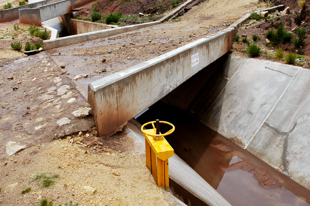
4.  APPLICATION TO IMPERIAL VALLEY CANAL DATA

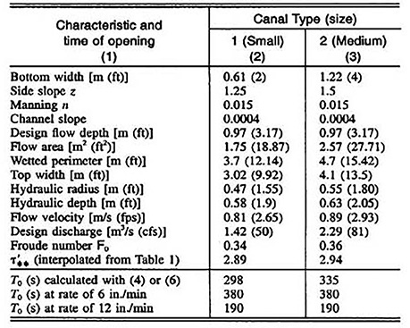
The developed criterion (Eqs. 4-6) is applied to two typical irrigation canal designs in the Imperial Valley, California. The hydraulic data were supplied by the Imperial Irrigation District's Engineering Division in Brawley, Imperial County. Canal 1 is small, with a 2-ft bottom width; Canal 2 is medium-sized, with a 4-ft bottom width. The hydraulic characteristics are shown in Table 2, together with the time of opening calculated using Eq. 5 or 6. Also shown is the actual time of opening, based on two rates-of-rise recommended by the manufacturers, 15.24 cm/min (6 in/min) and 30.48 cm/min (12 in/min). It is seen that actual and calculated times-of-opening are in reasonable agreement, as the theoretically calculated value lies between the two rates established by practice. Accordingly, Eq. 4 or its surrogate equations (Eqs. 5 and 6), is proposed as an indicator of the time of opening of irrigation canal gates in field situations of comparable hydraulics and geometry. The proposed methodology is applicable provided the transients generated by the gate operation are of small amplitude.