1. INTRODUCTION
The stability and convergence properties of explicit numerical schemes of the pure convection equation have been known for some time. A unified theoretical treatment is presented herein.
2. PURE CONVECTION EQUATION The pure convection equation is of the following form:
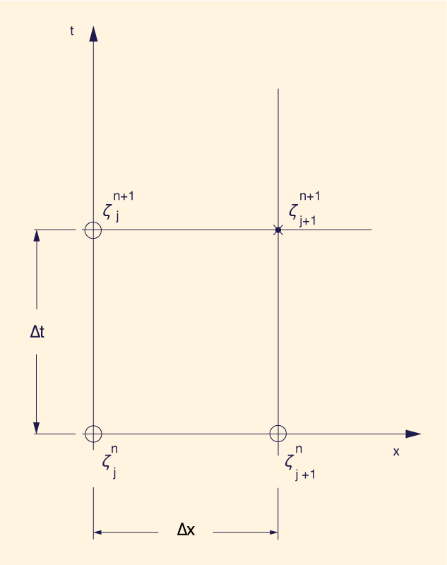
in which ζ = any physical quantity to be convected with the velocity u. A general explicit finite difference scheme of this equation is as follows (Fig. 1):
in which X and Y = weighting factors of the temporal and spatial derivatives, respectively; Δt and
In Equation 2, solving explicitly for the unknown value ζ j+1 n+1 gives:
in which:
and
is the Courant number corresponding to the particular grid location. 3. NUMERICAL DIFFUSION COEFFICIENT Equation 1 is an inviscid equation, therefore, viscosity (or diffusivity, as the case may be) is absent from it. However, a numerical solution of Eq. 1 will often show a viscous (diffusive) behavior. This is to be correctly attributed to the artificial viscosity of the scheme itself. The term "numerical dispersion" is sometimes used in this connection, ostensibly to denote the fact that both amplitude and phase errors aggregate to produce a dispersive type of effect in the numerical solution. A measure of the amount of numerical dispersion can be obtained from the approximation error of the finite difference scheme. This can be obtained by expanding the grid function ζ(jΔx, nΔt) as a Taylor series about point jΔx, nΔt, leading to (1,2):
in which R = the approximation error. From Eq. 8, for X = Y = 1/2, the scheme is of second-order accuracy. i.e., R = ο(Δx2). In addition, for C = 1, the accuracy is at least of third order. In fact, for these conditions the exact solution is obtained (1). The coefficient of the term ∂2ζ / ∂x2 in Eq. 8 is referred to as the numerical diffusion coefficient, μn, defined as follows:
Positive values of μn cause the wave amplitude to diffuse numerically; negative values cause the wave amplitude to amplify numerically. While in the former the consistency is impaired, in the latter stability suffers. Both stability and consistency improve as μn approaches zero. Table 1 summarizes the stability and convergence (consistency in the limit) properties of three common first-order schemes.
4. VON NEUMANN LINEAR ANALYSIS A considerable insight into the numerical properties of the various four-point explicit schemes for the computation of pure convection can be gained by a linear analysis of stability and convergence following the von Neumann approach (3,4). According to this method, a solution of Eq. 2 is sought in sinusoidal form:
in which ζο = an amplitude function; σ = wave number of the sinusoidal solution; and β = complex propagation factor, such that β = βR + i βI. The quantity βR = wave frequency; and βI = amplification (or attenuation) factor. The substitution of Eq. 10 into Eq. 2 leads to:
Substituing exp (i σ Δx) = p + i q, in which p = cos (σΔx) and q = sin (σΔx) into Eq. 11 leads to:
in which:
Operating on Eq. 12:
in which:
and
Separating Eq. 15 into its real and imaginary components:
Since the analytical solution of Eq. 1 exhibits no damping, it follows that Eq. 20 is a measure of numerical damping (or amplification) of the numerical solution after one time increment Δt.
From Equation 19, the phase velocity of the numerical solution is:
A convergence ratio with regard to wave phase is defined as follows:
or likewise:
in which σΔx = the spatial resolution. Since σ = 2 π /L, in which L is the sinusoidal wavelength, it follows that:
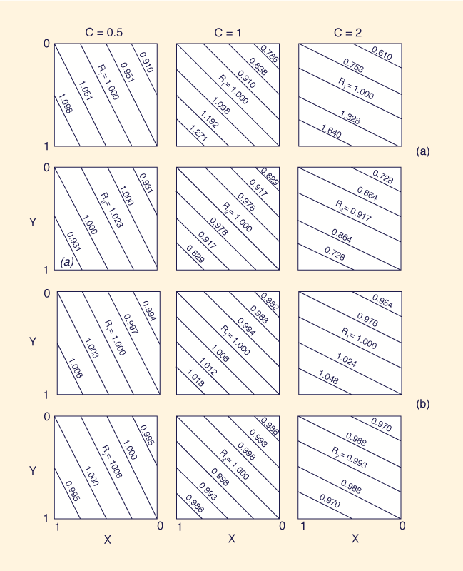
in which L / Δx is the number of discrete space intervals per sinusoidal wavelength. Both R1 and R2 are functions of X, Y, C, and L / Δx. Fig. 2 shows the variation of R1 and R2 as a function of X, Y, C, and L / Δx. The following conclusions can be obtained from this figure:
The instability, R1 > 1, of Scheme I (Table I) for Courant numbers greater than 1, and of Scheme II for Courant numbers less than 1, is confirmed. Likewise, the unconditional stability and stronger numerical dispersion of Scheme III is confirmed.
5. STABILITY AND CONVERGENCE PROPERTIES Linear equation with constant coefficient. In this case, the convective velocity u is constant in space and time. The numerical solution using Eqs. 3-6 with X = Y = 1/2 and C = u Δt / Δx = 1 will exactly reproduce the analytical solution.
Linear equation with variable coefficient. In this case, the convective velocity u varies in space and time. Therefore, the Courant number varies from one computational cell to the next. The stability of the scheme requires that μ ≥ 0; on the other hand. convergence of the wave amplitude improves as μn → 0. Using Eq. 9, several unconditionally stable yet second-order accurate explicit schemes can be formulated. The numerical properties of three of these schemes are given in Table 2. Schemes IV and V can be regarded as generalizations of Schemes I and II, respectively, for the case of varying Courant numbers. However, unlike Schemes I and II, Schemes IV and V do not diffuse the wave amplitude numerically. Scheme VI, a space-and-time centered scheme, has second-order accuracy for all C. For fixed values of X and Y the second-order error of Schemes IV to VI will be directly proportional to | 1 - C |. Likewise, for fixed values of X, Y and C (C ≠ 1), the second-order error will be directly proportional to ∂3 ζ / ∂x 3. The equivalence of Schemes IV to VI can be demonstrated by substituting the values of X and Y of Table 2 into Eqs. 4-6. This leads to:
and
for all three schemes. Furthermore, for C = 1, C2 = C3 = 0, and ζ j + 1 n + 1 = ζj n, i.e., the quantity ζ is being subjected to pure convection. For C ≠ 1 a dispersive effect is introduced because the calculation of ζ j + 1 n + 1 is being based not only on ζj n but also on ζj n + 1 and ζj + 1 n . 6. ILLUSTRATIVE EXAMPLE
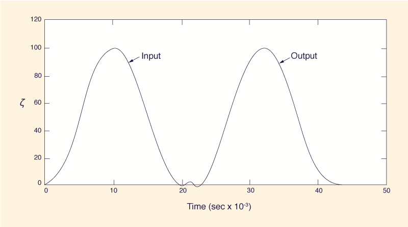
A hypothetical example was set up to demonstrate the numerical properties of the schemes described in Table 2. A channel 20,000 ft long was divided into 20 reaches of Δx = 1,000 ft The results of the simulation are shown in Fig. 3. Stability, convergence of the wave amplitude, and mass conservation are maintained for all Courant numbers. Predictably, a small amount of numerical noise was detected.
This is caused by the second-order errors, and tends to be concentrated in the regions of sharp changes in ∂3ζ /∂x3 (or ∂3ζ /∂t 3).
The numerical error is a function of | 1 - C | and
vanishes as
7. SUMMARY AND CONCLUSIONS A unified theoretical treatment of the numerical properties of a class of explicit schemes of the pure convection equation is presented. For the cases of slowly varying Courant numbers, the theory is used to show that unconditional stability and second-order accuracy can be achieved within the framework of an explicit formulation. APPENDIX |. REFERENCES
APPENDIX ||. NOTATION C = Courant number; C1 = coefficient, Eq. 4; C2 = coefficient, Eq. 5; C3 = coefficient, Eq. 6; j = space discretization index; L = wavelength; M = parameter, Eq. 16; N = parameter, Eq. 17; n = time discretization index; P = parameter, Eq. 18; p = cos (σΔx); q = sin (σΔx); R = approximation error; also, parameter, Eq. 13; R1 = wave amplitude convergence ratio; R2 = wave phase convergence ratio; S = parameter, Eq. 14; u = mean velocity; μn = phase velocity of numerical solution; X = weighting factor of temporal derivative; Y = weighting factor of spatial derivative; βI = amplification (or attenuation) factor; βR = wave frequency; Δt = temporal increment; Δx = spatial increment; ζ = any physical quantity to be convected; μn = numerical diffusion coefficient, Eq. 9; and σ = wave number.
| ||||||||||||||||||||||||||||||||||||||||||||||||||||||||||||||||||||||||||||||||||||||||||||||||||||||||||||||||||||||||||||||||||||
| 220525 |
| Documents in Portable Document Format (PDF) require Adobe Acrobat Reader 5.0 or higher to view; download Adobe Acrobat Reader. |