1. INTRODUCTION
The Muskingum-Cunge method of flood routing is well established in the hydrologic
engineering literature (Cunge, 1969; Ponce and Yevjevich, 1978; U.S. Army
Corps of Engineers, 1990). It is a convenient method because the routing parameters
are a function of channel properties and grid specification, which leads to results
which are independent of grid size. The method has linear and nonlinear modes. In
the linear mode, average flow values are used to calculate the routing parameters at
the start of the computation, and these are kept constant throughout the computation
in time. In the nonlinear mode, the routing parameters are recalculated for every
computational cell as a function of local flow values.
Both modes of computation have their advantages and disadvantages. The linear
mode conserves mass, but it requires a priori estimation of a reference flow on which
to base the computation of the routing parameters. In addition, the routed flows lack
the steepening exhibited by inbank flood waves. Conversely, the nonlinear mode does
not require the specification of a reference flow and can simulate the wave steepening.
Unfortunately, the nonlinear mode is saddled with a small but perceptible loss of
mass.
Given the trade-offs involved, it seems certain that both routing modes will
continue to be used in the future. The linear mode will be used where simplicity is desired,
notwithstanding its lack of wave steepening. The nonlinear mode will be used where
the simulation of wave steepening is judged to be important, albeit at the cost of a
small loss of mass. A multilinear method, representing a compromise between linear
and nonlinear methods, has been developed recently by Perumal (1992).
The Muskingum-Cunge is a viable alternative to the classical Muskingum method,
particularly for the cases where hydrologic data (i.e., streamflow data) are not available,
but where hydraulic data (cross-sectional data and channel slopes) can be
readily ascertained. In many instances, the Muskingum-Cunge method is also an
alternative to the more complex dynamic wave models, which lack robustness and
have significant data requirements. The nonlinear features of the variable-parameter
Muskingum-Gunge method makes it the method of choice in hydrologic flood
routing.
This paper revisits the variable-parameter Muskingum-Cunge method of Ponce
and Yevjevich (1978). The small but perceptible loss of mass is confirmed throughout
a wide range of unit peak inflows, from 200 to 1000 cfs ft-1 (18.58-92.9 m-2s-1).
Furthermore, a slight improvement in mass conservation is realized by an alternative way of
calculating the variable parameters.
2. BACKGROUND
The Muskingum-Cunge method is a variant of the Muskingum method (Chow,
1959) developed by Cunge (1969) and documented in the Flood Studies Report
(Natural Environment Research Council, 1975). Ponce and Yevjevich (1978)
expressed the routing parameters of the Muskingum-Cunge method in terms of
the Courant and cell Reynolds numbers, two physically and numerically meaningful
parameters. In addition, they developed a nonlinear mode of calculating the parameters,
thereby enhancing the method's applicability to real-world routing problems.
A three-point method and an iterative four-point method were suggested as a way to
vary the parameters as a function of local flow values. The method has been adopted
by the most recent version (Version 4.0) of the US Corps of Engineers' HEC-1 model
(1990).
The routing equation of the Muskingum-Cunge method defined in the typical
four-point grid configuration is:
in which j is a spatial index, n is a temporal index, and:
C0 = (-1 + C + D) / (1 + C + D)
C1 = (1 + C - D) / (1 + C + D)
C2 = (1 - C + D) / (1 + C + D)
are the routing coefficients, with C the Courant number, defined as follows:
C = c (Δt / Δx)
in which c is the wave cerelity, Δt is the time interval, Δx is the space interval, and D the cell Reynolds number, defined as follows:
D = q /(So c Δx)
in which q is the unit-width discharge and So is the bottom slope.
The wave celerity is defined as follows:
c = β (Q /A) = β (q / d )
in which β is the exponent of the rating, A is the flow area, and d is the flow depth.
The Muskingum-Cunge method matches the numerical diffusion of the discrete
model with the physical diffusion of the analytical model. The advantage is that the
routing results are independent of the grid specification, provided numerical dispersion
is minimized. The numerical dispersion can be minimized by keeping the
Courant number equal to or slightly greater than one (Cunge, 1969; Ponce and
Theurer, 1982; Ferrick et. al., 1983).
3. NUMERICAL EXPERIMENTS
In this paper, Thomas' (1934) classical problem was chosen to test the
Muskingum-Cunge method under a wide range of flow conditions. The Thomas
problem was chosen here to allow comparison with previous results (Ponce and
Yevjevich, 1978). The original problem considered routing a sinusoidal flood wave
with a 96-h period through a prismatic channel 500 miles long. A unit-width channel
of baseflow qb = 50 cfs ft-1 (4.64 m2 s-1) and peak inflow qpi = 200 cfs ft-1 (18.58 m2 s-1) was specified. The bottom slope was set at 1 ft mile-1, and the discharge-depth rating was the following:
q = 0.688 d 5/3
This amounts to a Manning's n = 0.0297. It can be shown that the 96-h sinusoidal
flood wave satisfies the diffusion wave applicability criterion (Ponce et. al., 1978).
The following methods are considered here:
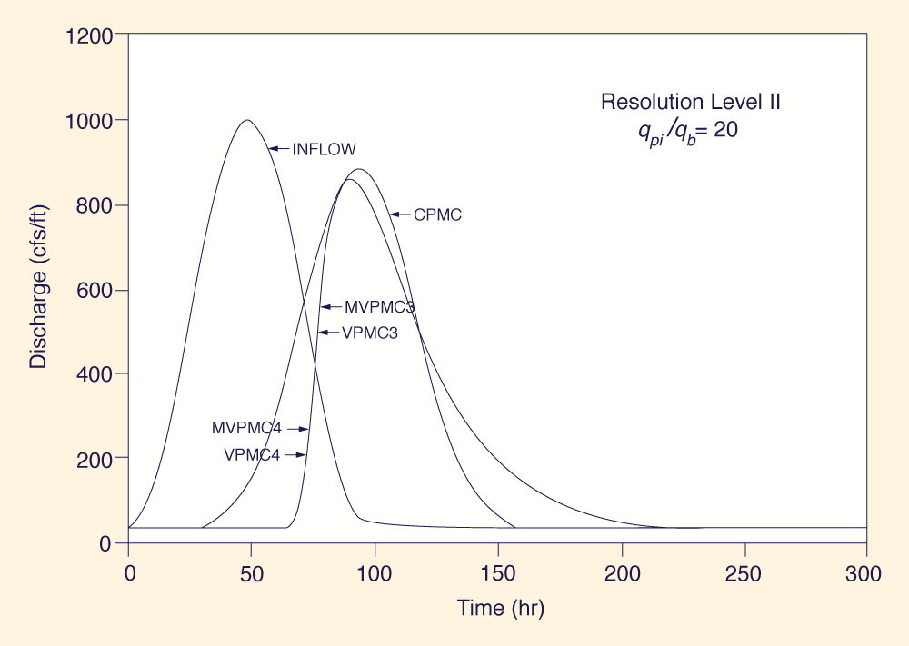
The constant-parameter method (CPMC), in which the routing parameters C
and D are the same for all computational cells. They are based on an average unit-width discharge qa calculated as:
qa = (qb + qpi) / 2
The average celerity ca is calculated with Eq. 7, using the discharge computed with Eq. 9.
The three-point variable-parameter method (VPMC3) (Ponce and Yevjevich,
1978), in which the routing parameters C and D for each computational cell are based
on the average unit-width discharge and celerity at the three known grid points:
The iterative four-point variable-parameter method (VPMC4) (Ponce and
Yevjevich, 1978), in which the routing parameters C and D for each computational
cell are based on the average unit-width discharge and celerity at the four
grid points:
To improve the convergence of the iterative procedure, the discharge qj + 1n + 1 obtained
with the three-point method (VPMC3) is used as a first guess of the iteration. The
celerity
A modified three-point variable-parameter method (MVPMC3), in which the
routing parameters C and D for each computational cell are based on the average
unit-width discharge at the three known grid points:
Unlike the VPMC3, the average celerity c a is calculated with Eq. 7, based on the
discharge computed with Eq. 14.
A modified iterative four-point variable-parameter method (MVPMC4), in
which the routing parameters C and D for each computational cell are based on
the average unit-width discharge at the four grid points:
Unlike the VPMC4, the average celerity c a is calculated with Eq. 7, based on the
discharge qa computed with Eq. 15. To improve the convergence of the iterative
procedure, the discharge
Two levels of spatial and temporal resolution were chosen:
Resolution level I, the grid specification used by Thomas (1934): Δx = 25 miles
(40.22 km), and Δt = 6 h; and
Resolution level II, a finer grid specification used in this
paper: Δx = 12.5 miles (20.11 km), and Δt = 3 h.
Three peak inflow to baseflow ratios qpi /qb were used:
qpi /qb = 4, used by Thomas (1934), Dooge
(1973), and Ponce and Yevjevich (1978);
qpi /qb = 10; and
qpi /qb = 20.
These peak
inflow to baseflow ratios encompass a wide range of practical values. With
qpi
4. RESULTS
The mass conservation properties were assessed by integrating inflow and outflow
hydrographs for the 500-mile reach. Table 1 shows peak outflow qpo, ratio of peak
outflow to peak inflow
The following conclusions are drawn from Table 1:
It should be noted that the mass conservation percentages shown in Column 7 of Table 1 are cumulative values for the 500-mile reach of the Thomas problem. A typical flood routing application would normally not consider such long reach without intervening lateral inflows which tend to mask the accuracy of the computation. Therefore, the percentages shown should be interpreted as an extreme or worst-case scenario.
Figure 1 shows a set of flood hydrographs for resolution level II and peak inflow to
baseflow
5. CONCLUSIONS The modified variable-parameter methods MVPMC3 and MVPMC4 developed in this paper result in a definite improvement in mass conservation, as compared with the conventional methods VPMC3 and VPMC4 (Ponce and Yevjevich, 1978). The improvement may be more marked when using a wide range of realistic discharges. Otherwise, the small loss of mass does not appear to impose a significant drawback. It is the price to be paid to model the nonlinear features of a flood wave within the framework of the Muskingum-Cunge method. REFERENCES Chow, V. T., 1959. Open-Channel Hydraulics. McGraw-Hill, New York.
Cunge, J. A., 1969. On the subject of a flood propagation computation method (Muskingum method). J. Hydraul. Res., 7(2) 205-230.
Dooge, J. C. I., 1973. Linear theory of hydrologic systems. U.S. Dep. Agric. Tech. Bull., 1468, 327 pp.
Ferrick, M. G., Bilmes, J. and Long, S. E., 1983. Modeling rapidly varied flow in tailwaters. Water Resour. Res., 20(2): 271-289.
Natural Environment Research Council, 1975. Flood Studies Report, Vol. III. Natural Environment Research Council, London.
Perumal, M., 1992. Multilinear Muskingum flood routing method. J. Hydrol., 133: 259-272.
Ponce, V. M. and Theurer, F. D., 1982. Accuracy criteria in diffusion routing. J. Hydraul. Div., ASCE., 108 (HY6): 747-757.
Ponce, V. M. and Yevjevich, V., 1978. Muskingum-Cunge method with variable parameters. J. Hydraul. Div. ASCE, 104(HY12): 1663-1667.
Ponce, V. M., Li, R-M. and Simons, D. B., 1978. Applicability of knematic and diffusion models. J. Hydraul. Div. ASCE, 104(HY3): 353-360.
Thomas, H. A., 1934. The hydraulics of flood movement in rivers. Eng. Bull., Carnegie Inst. of Technology, Pittsburgh, PA.
US Army Corps of Engineers, 1990. HEC-1, flood hydrograph package: User's manual, version 4, 1990. US Army Corps of Engineers, Hydrologic Engineering Center, Davis, CA.
| |||||||||||||||||||||||||||||||||||||||||||||||||||||||||||||||||||||||||||||||||||||||||||||||||||||||||||||||||||||||||||||||||||||||||||||||||||||||||||||||||||||||||||||||||||||||||||||||||||||||||||||||||||||||||||||||||||||||||||||||||||||||||||||||||||||||||||||||||||||||||||||||||||||||||||||||||
| 211229 |
| Documents in Portable Document Format (PDF) require Adobe Acrobat Reader 5.0 or higher to view; download Adobe Acrobat Reader. |