KINEMATIC AND DYNAMIC HYDRAULIC DIFFUSIVITIES USING SCRIPT ONLINEOVERLAND
1. INTRODUCTION
In diffusion wave modeling of catchment dynamics,
the hydraulic diffusivity may be expressed in two alternative ways:
(1) kinematic; or (2) dynamic. The kinematic hydraulic diffusivity
is due to Hayami (1951), who pioneered the diffusion wave approach
to surface flow. An extension of the concept
of hydraulic diffusivity to the domain of dynamic waves
followed, notably first by Dooge and his collaborators
(Dooge, 1973;
Dooge et al., 1982),
and later by Ponce (1991a;
1991b).
The kinematic hydraulic diffusivity is
(Hayami, 1951):
in which qo = reference unit-width discharge, and So = bottom slope.
Dooge (1973) extended the concept of hydraulic diffusivity to the realm of
dynamic waves by incorporating the
dependency of the hydraulic diffusivity on
the Froude number F, as follows:
in which νd = dynamic hydraulic diffusivity.
Subsequenty,
Dooge et al. (1982) expressed the dynamic hydraulic
diffusivity in terms of the exponent β of
the discharge-area rating curve, wherein Q = α A β.
The enhanced formulation is the following:
Ponce
(1991a;
1991b)
expressed the dynamic hydraulic diffusivity in terms
of the Vedernikov number:
in which the Vedernikov number is:
While the kinematic
hydraulic diffusivity (Eq. 1) is independent
of the Froude and/or Vedernikov numbers, the dynamic
hydraulic diffusivity (Eq. 4)
has a clearly defined threshold for V = 1, being positive for
This paper sheds light on the role of the Vedernikov number in catchment dynamics. The specific
question to be answered is the following:
How important is the dynamic hydraulic diffusivity (Eq. 4)
in affecting
catchment response, under a wide range of flow conditions?
We explore this question by using the script ONLINEOVERLAND,
an analytical tool capable of considering either the kinematic (Eq. 1) or dynamic (Eq. 4)
approaches to model hydraulic diffusivity.
The conclusions may prove of interest to engineers and scientists
engaged in diffusion wave modeling
of catchment dynamics.
2. OVERLAND FLOW MODELING
Overland flow is surface runoff that flows across the land
immediately following a rainfall event.
The diffusion wave model is an improvement over the conventional
kinematic wave model
because it is grid independent. This property reflects the model's
ability to provide essentially the same result,
regardless of grid size. This significant feature,
which sets the diffusion wave model
apart from conventional overland flow models, is obtained
by matching physical and numerical diffusivities
(Cunge, 1969;
Ponce, 1986). In addition to matching
diffusivities, ONLINEOVERLAND
effectively minimizes numerical
dispersion, i.e., the third-order discretization error,
by defining the grid ratio
such that the Courant number, in planes and channel,
is as
3. TEST PROBLEM
A reference test problem was chosen for use together
with script ONLINEOVERLAND.
For a given overland flow modeling problem,
the script requires the input of twenty-four (24)
parameters, which, taken as a set, describe the geometric and physical characteristics
of the overland flow problem.
These parameters are selected to perform sensitivity analysis. The objective is to
determine the difference in catchment response (i.e., the outflow hydrograph), between the two types of
hydraulic diffusivities considered here: (1) kinematic (Eq. 1); and (2) dynamic (Eq. 4).
The results of the sensitivity analysis are presented in Sections 4 to 7.
4. EFFECT OF DRAINAGE AREA
In this section we describe the response of the diffusion
wave model of catchment dynamics to the variation of drainage area, i.e.,
the overland flow area A (Table 1, row 11).
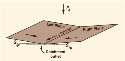
We note that the response of the reference test problem (Section 3)
is a superconcentrated catchment flow hydrograph, wherein the
rainfall duration (12 hr) exceeds the time of concentration
(Ponce, 2014a;
2014b).
ie = P/tr = 24 cm / 12 hr = 2 cm/hr.
Qp = ie A =
2 cm/hr × 18 ha = 1 m3/s.
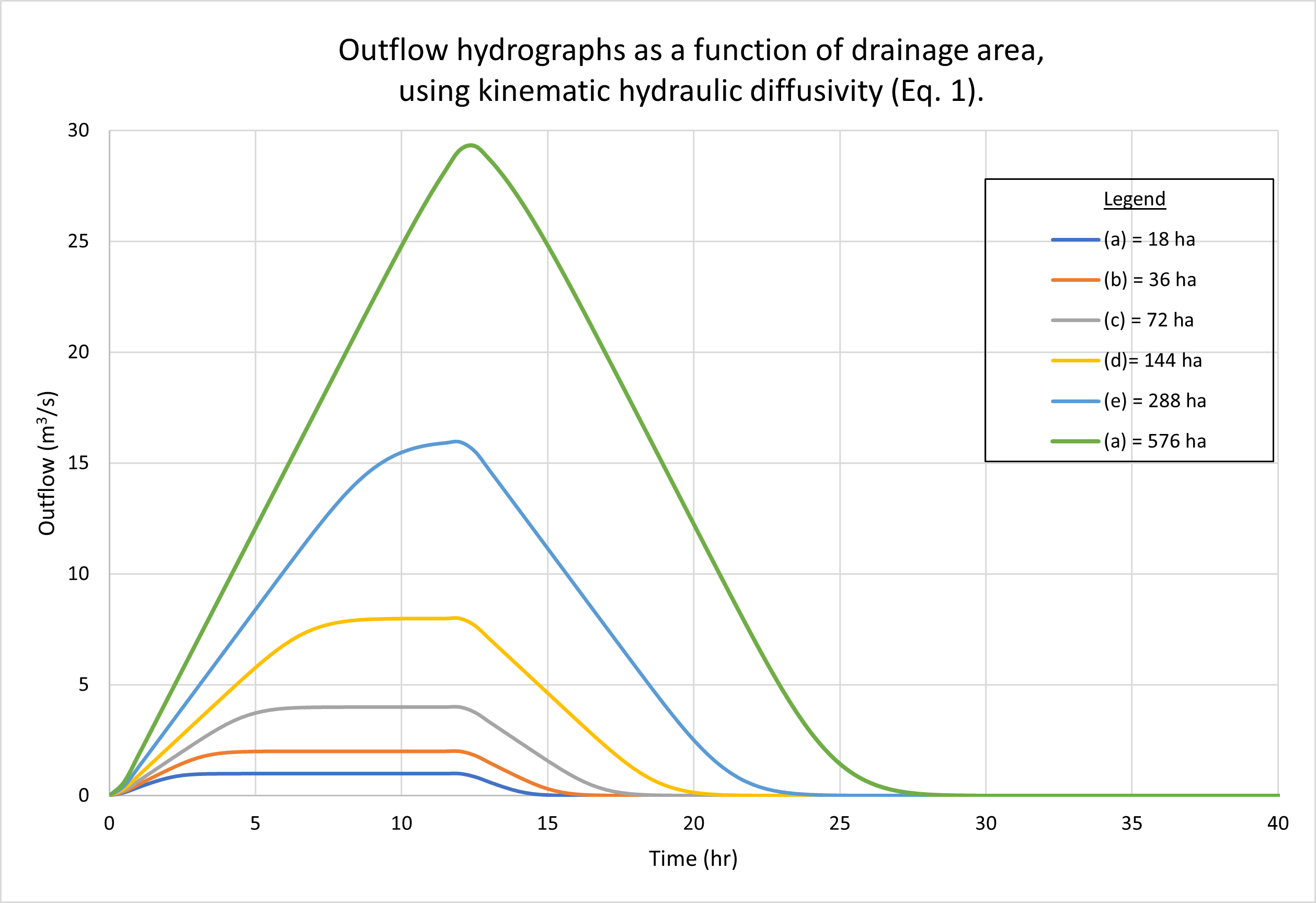
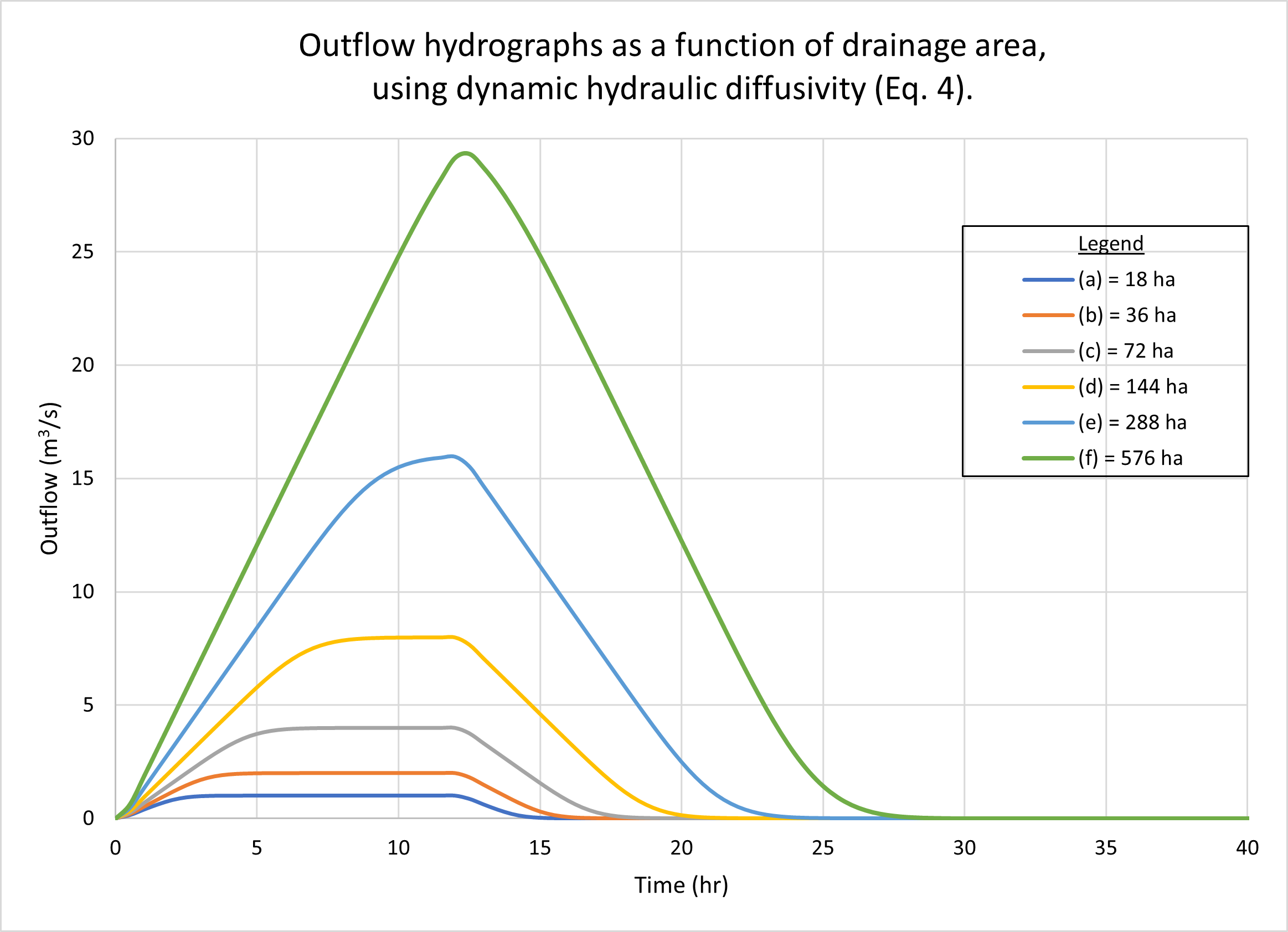
Figure 2 shows the hydrographs calculated by ONLINEOVERLAND
for a series of drainage areas, each determined by doubling the
previous value, starting with the reference test problem
of 18 ha, as follows: (a) 18 ha; (b) 36 ha; (c) 72 ha; (d) 144 ha; (e) 288 ha, and (f)
576 ha. Figure 2 (a) shows the results using the kinematic hydraulic diffusivity (Eq. 1).
Fig. 2 (b) shows the results using the dynamic hydraulic diffusivity (Eq. 4).
No appreciable difference in catchment response may be observed
with the variation in drainage area.
We note that while hydrographs a, b, c, and d are superconcentrated,
featuring a typical flat top, hydrograph e is concentrated, with a distinct peak at
the maximum
possible (16 m3/s), while hydrograph f is subconcentrated, with its peak,
close to 29 m3/s,
falling short of reaching the maximum possible of
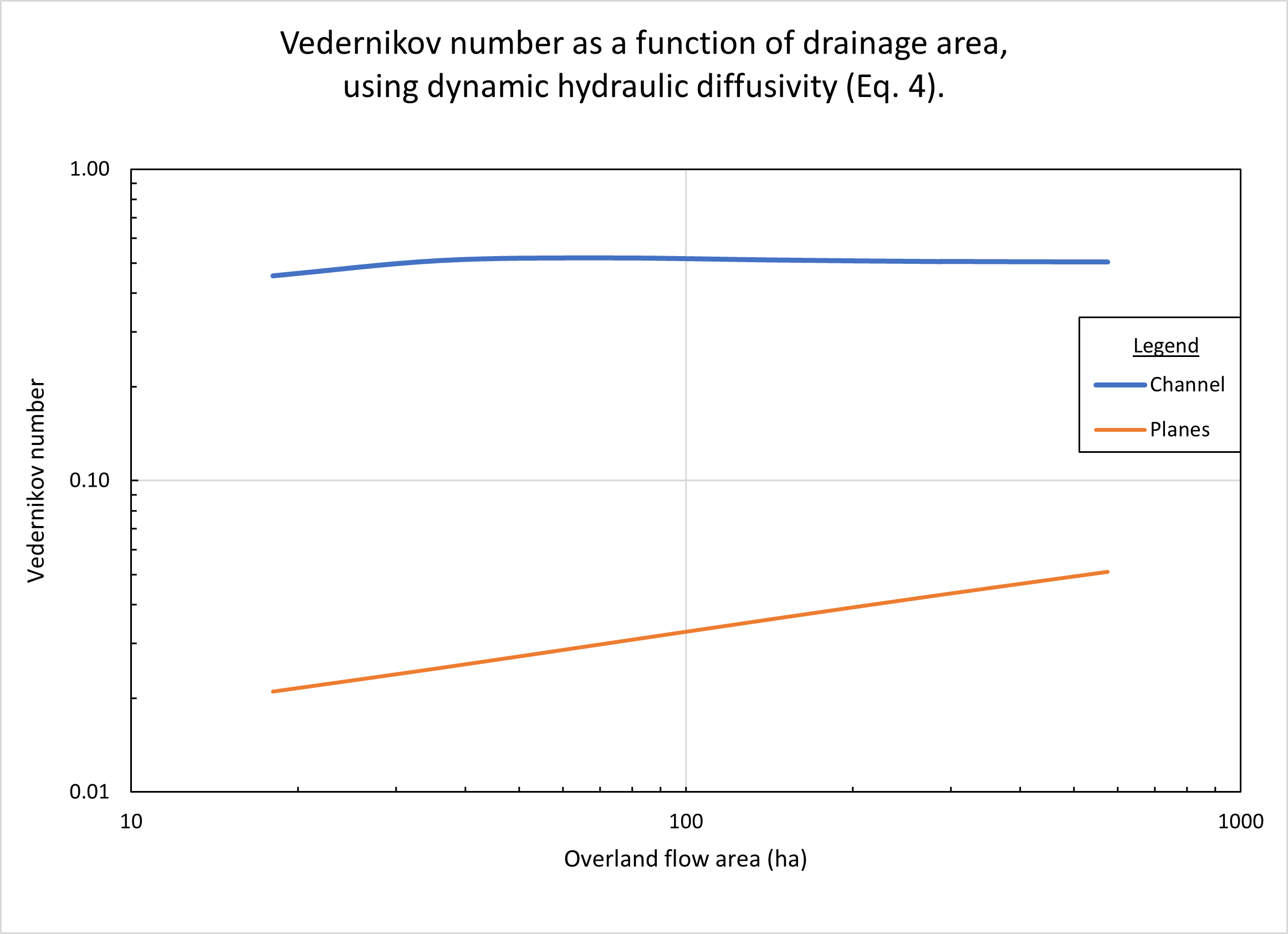
Figure 3 shows the calculated
Vedernikov number as a function of drainage area, using the dynamic hydraulic
diffusivity (Eq. 4). In order to accomodate the outflow for the
larger drainage areas, the design channel depth in the reference test problem
(Table 1, line 23) was increased to 1.2 m.
In the planes, the Vedernikov numbers are quite low,
increasing with an increase in drainage area A,
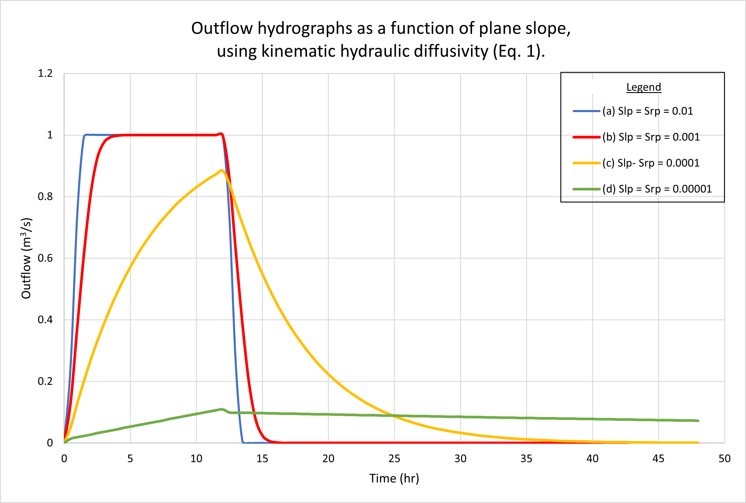
5. EFFECT OF PLANE SLOPE
In this section we describe the response of the diffusion wave model
of catchment dynamics to the variation of plane slopes, i.e.,
the slope of the left plane Slp (Table 1, row 13) and
the slope of the right plane Srp (Table 1, row 16).
In all cases, it is assumed that Srp
= Slp (reference test problem).
As with Section 4, the response
of the reference test problem is a superconcentrated
catchment flow hydrograph, wherein the rainfall duration (12 hr)
exceeds the time of concentration (Ponce, 2014).
ie = P/tr = 24 cm / 12 hr = 2 cm/hr.
Qp = ie A =
2 cm/hr × 18 ha = 1 m3/s.
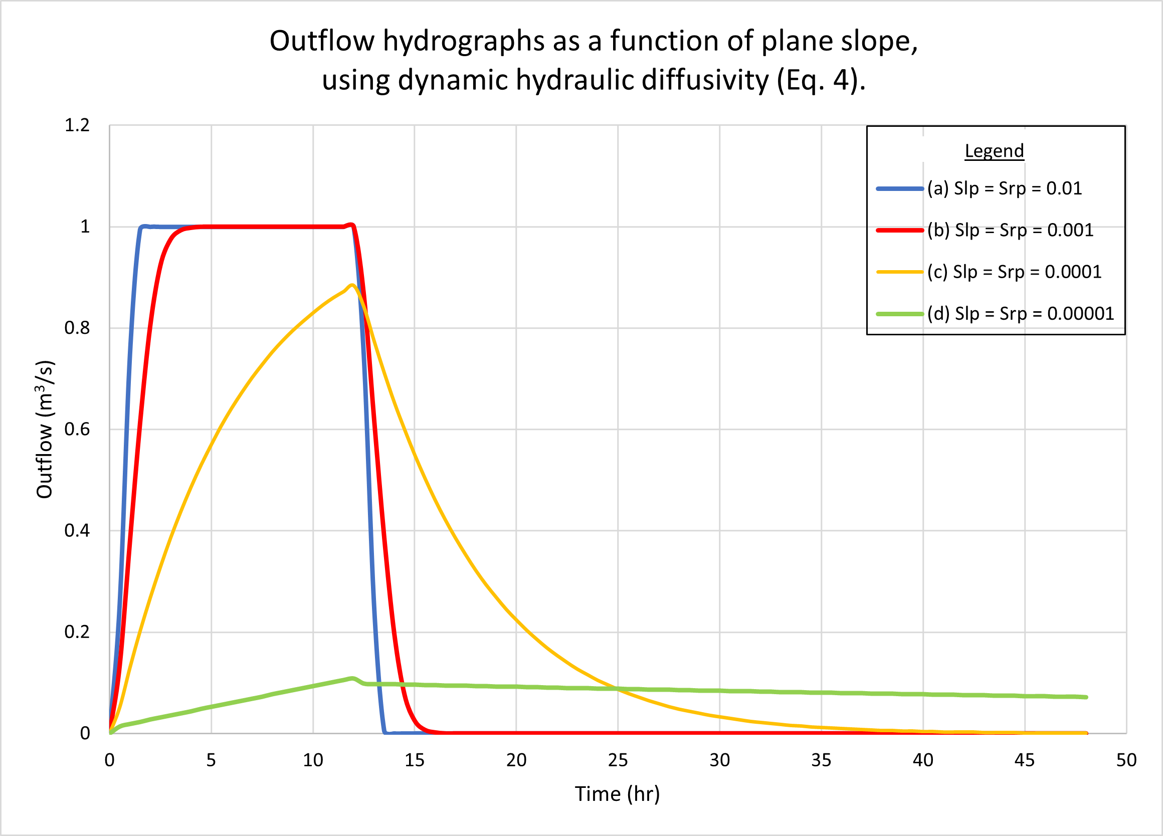
Figure 4 shows the hydrographs calculated by ONLINEOVERLAND
for four (4) plane slopes, as follows:
(a) 0.01; (b) 0.001; (c) 0.0001, and (d) 0.00001.
Figure 4 (a) shows the results using the kinematic hydraulic diffusivity (Eq. 1).
Fig. 4 (b) shows the results using the dynamic hydraulic diffusivity (Eq. 4).
No appreciable difference in catchment response between the two figures
may be observed.
As expected, hydrographs a and b are superconcentrated,
featuring the characteristic flat top at
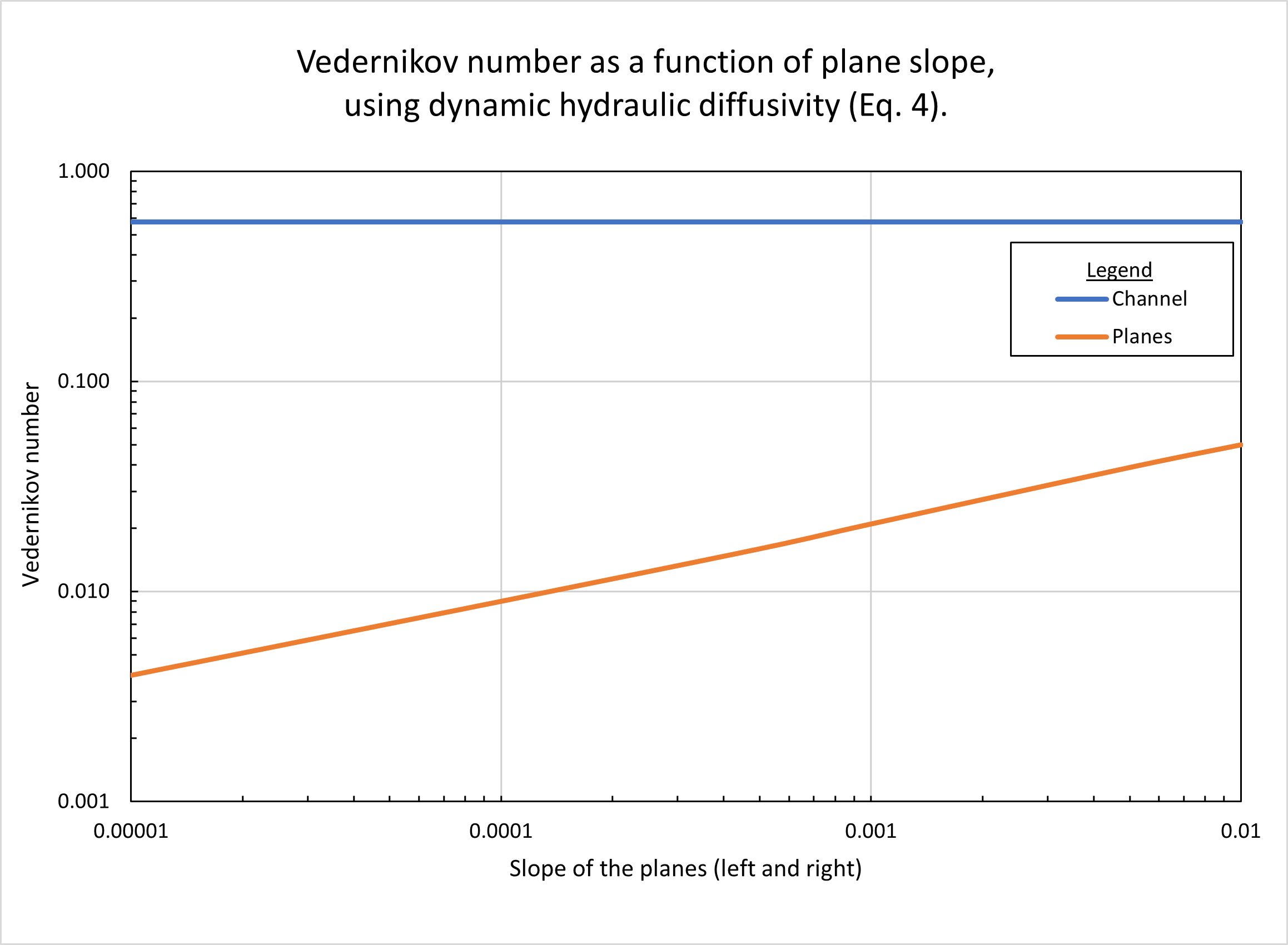
Figure 5 shows the calculated Vedernikov number, as a function of plane slope, using the dynamic hydraulic diffusivity (Eq. 4). In the planes, Vedernikov numbers are quite low, increasing with an increase in slope, from V = 0.004 for a slope Sp = 0.00001, to V = 0.05 for a slope Sp = 0.01. In the channel, the Vedernikov number is high (V = 0.58) and remains constant (with the variation in plane slope), since the relatively high channel slope (Sch = 0.01) is constant and corresponds to the reference test problem (Table 1, row 20).
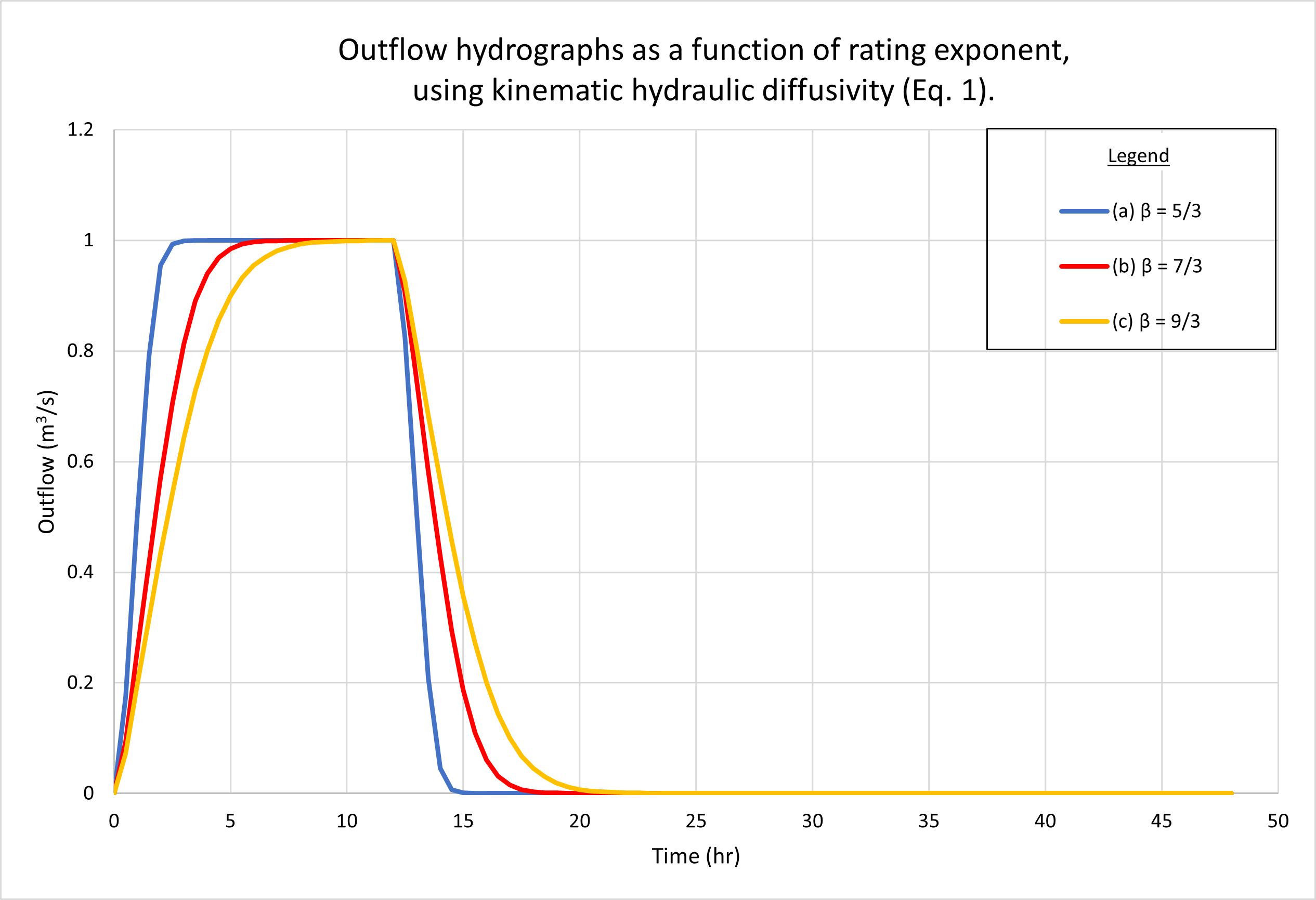
6. EFFECT OF RATING EXPONENT
In this section we describe the response of the
diffusion wave model of catchment dynamics to the variation in rating exponent
β. In free-surface flow, the latter varies with the type of friction and cross-sectional
shape (Ponce, 2014c).
We select three values of β, all three corresponding
to a hydraulically wide
channel, varying the
type of bottom friction as follows: (1) turbulent Manning, β = 5/3;
(2) mixed 50% laminar - 50% turbulent Manning, β = 7/3; and
(3) laminar, β = 9/3, i.e., β = 3.
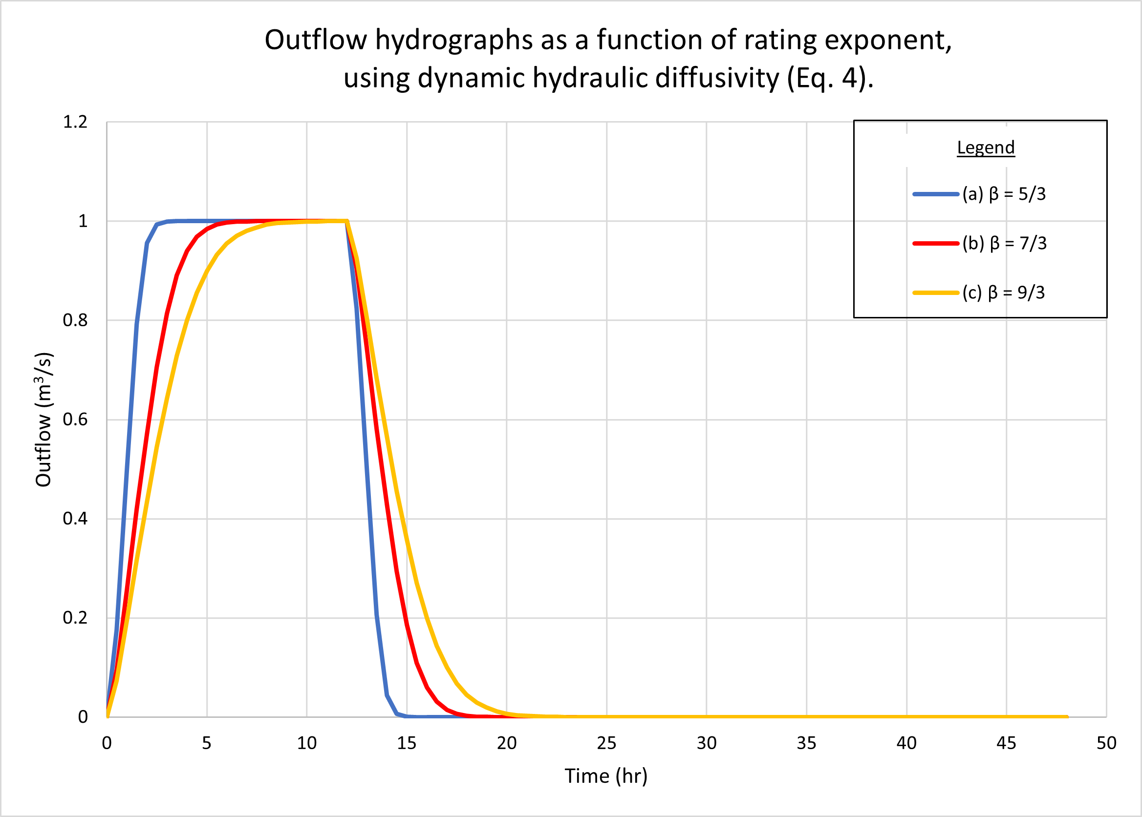
Figure 6 shows the hydrographs calculated by ONLINEOVERLAND.
Figure 6 (a) shows the results using the kinematic hydraulic diffusivity (Eq. 1).
Fig. 6 (b) shows the results using the dynamic hydraulic diffusivity (Eq. 4).
No appreciable difference in catchment response
between the two figures may be observed.
Note that all three hydrographs, a, b, and c,
are superconcentrated,
featuring the characteristic flat top at
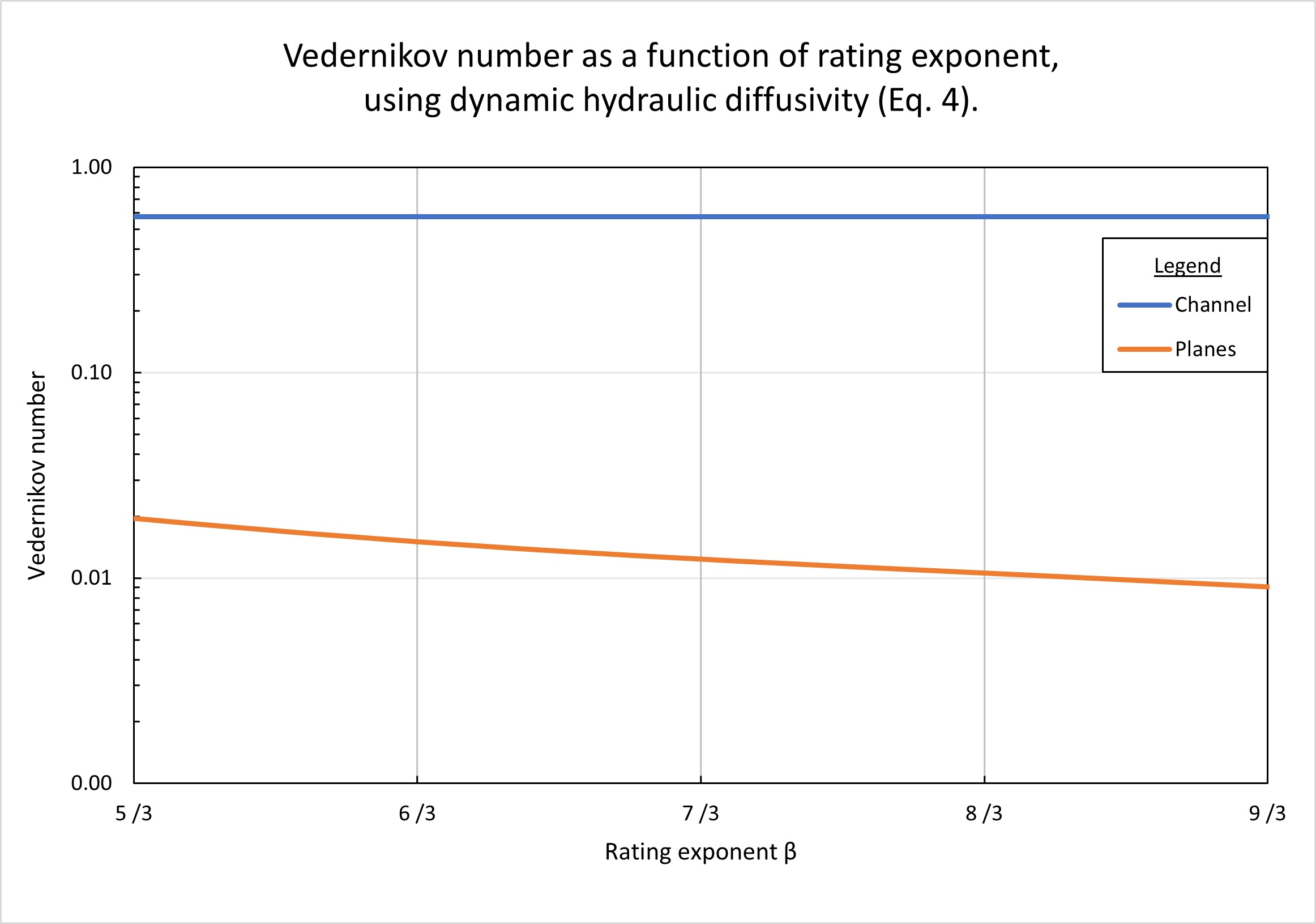
Figure 7 shows the calculated Vedernikov number as a function of rating exponent β, using the dynamic hydraulic diffusivity (Eq. 4). In the planes, Vedernikov numbers are quite low, decreasing with an increase in β, from V = 0.02 for β = 5/3 (turbulent Manning), to V = 0.0085 for β = 9/3 (laminar flow). In the channel, the Vedernikov number is high (V = 0.58) and remains constant (with the variation in rating exponent in the planes), since the relatively high channel slope (Sch = 0.01) is constant and corresponds to the reference test problem (Table 1, row 20).
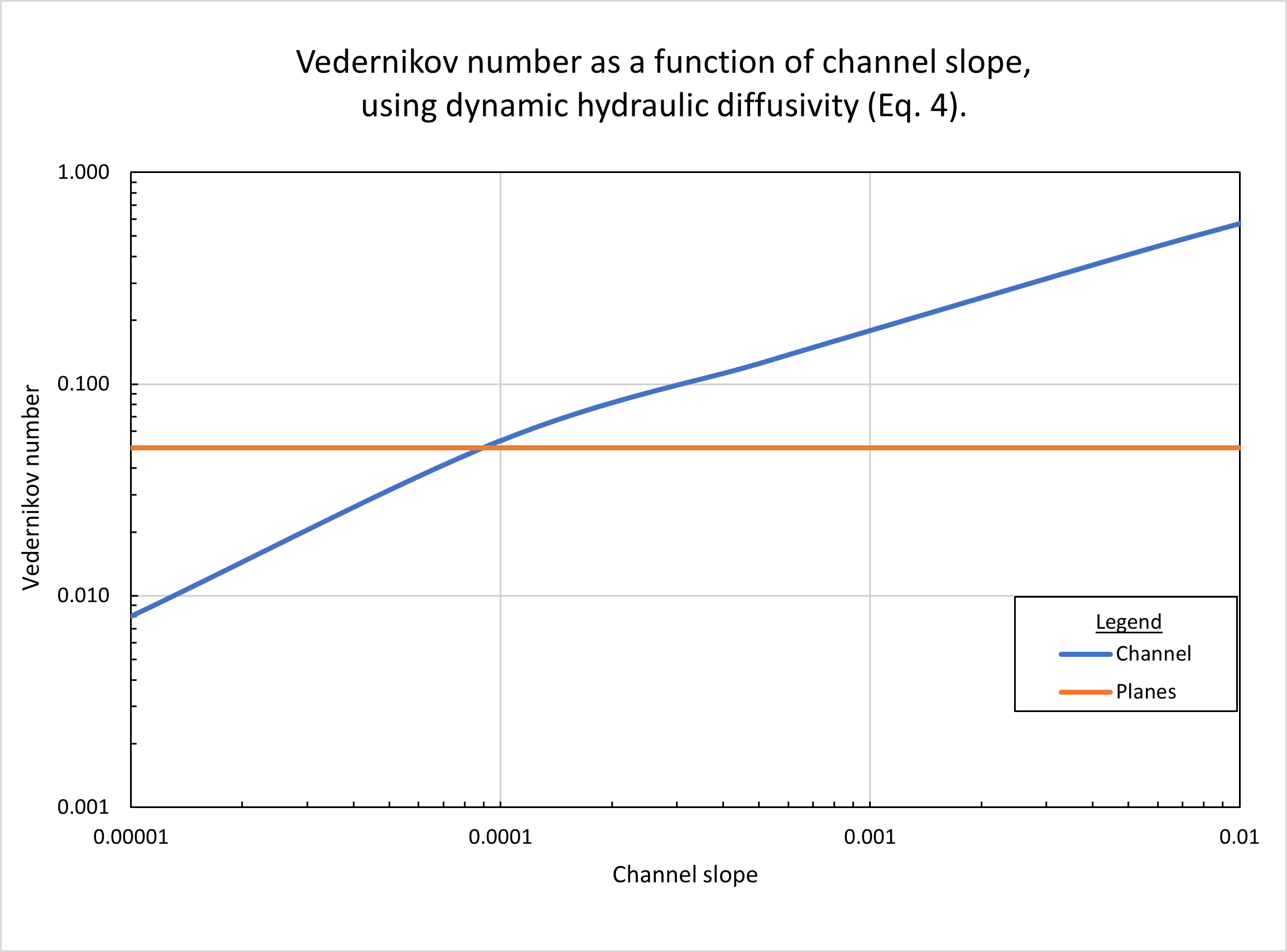
7. EFFECT OF CHANNEL SLOPE
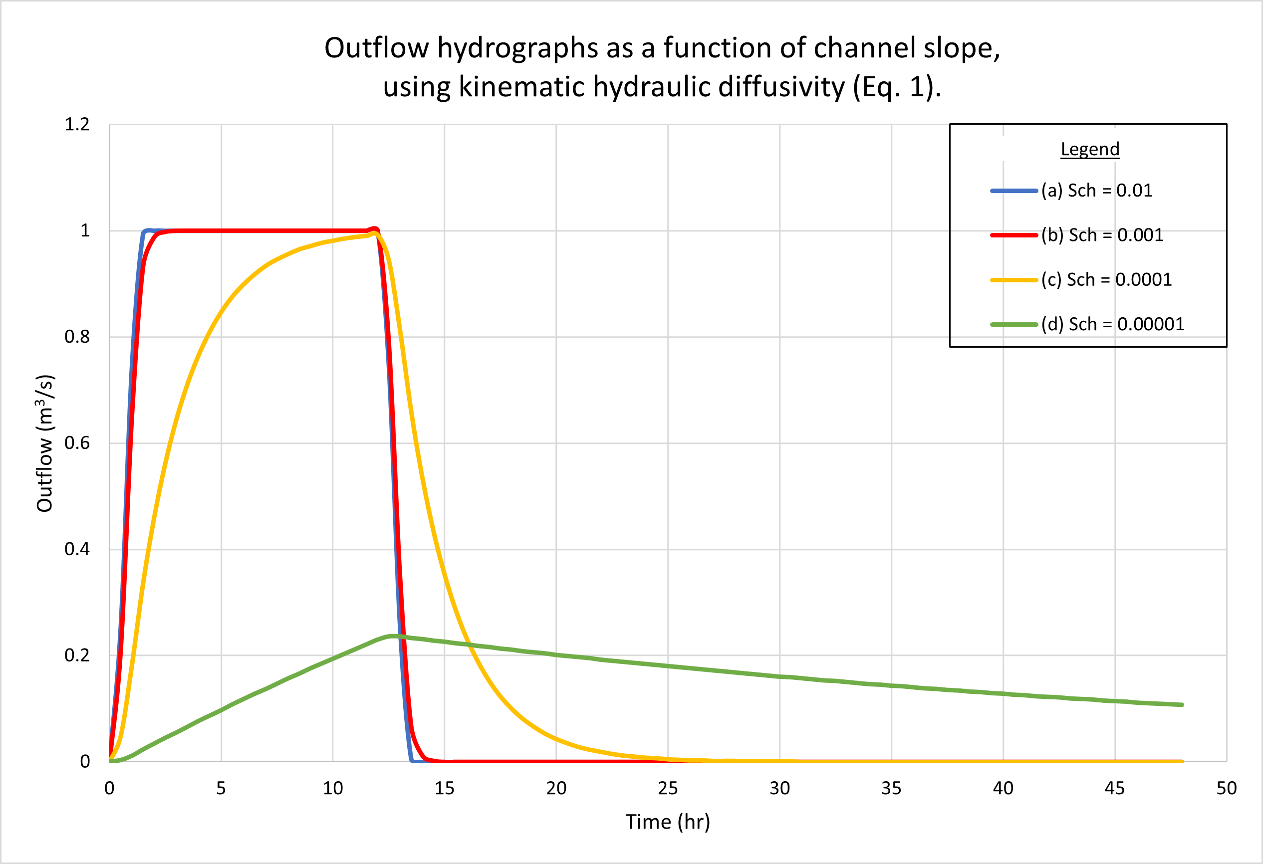
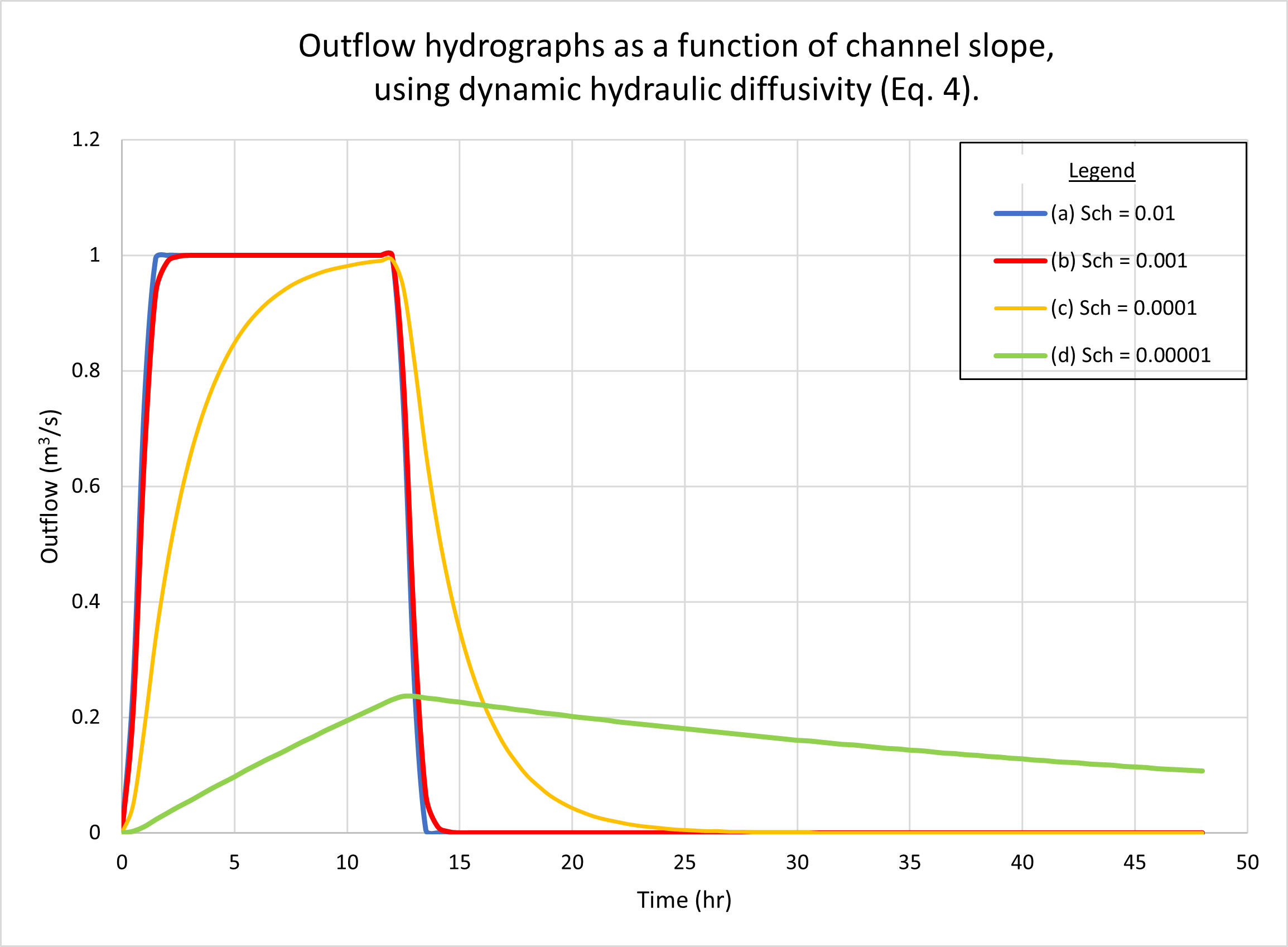
Figure 8 shows the hydrographs calculated by ONLINEOVERLAND
for four (4) channel slopes, as follows:
(a) 0.01; (b) 0.001; (c) 0.0001, and (d) 0.00001.
Figure 8 (a) shows the results using the kinematic hydraulic diffusivity (Eq. 1).
Fig. 8 (b) shows the results using the dynamic hydraulic diffusivity (Eq. 4).
No appreciable difference in catchment response between the two figures
may be observed.
As expected, hydrographs a and b are superconcentrated,
featuring the characteristic flat top at
Figure 9 shows the calculated
Vedernikov number as a function of channel slope,
using the dynamic hydraulic
diffusivity (Eq. 4).
In the planes, Vedernikov numbers remain constant and equal to
8. ANALYSIS The results of Sections 4 to 7 have clearly shown that the difference in outflow hydrographs between the two formulations for hydraulic diffusivity (kinematic, Eq. 1; and dynamic, Eq. 4), is negligible for the tested flow conditions listed in Table 1. The reason for this behavoir strikes at the core of shallow wave propagation mechanics (Ponce, 2019). Kinematic waves do not diffuse; therefore, for kinematic waves, any difference in the way diffusion is calculated (i.e., Eq. 1 vs. Eq. 4) would be negligible. Conversely, for diffusion waves, any difference in the way diffusion is calculated would be small. Furthermore, for mixed kinematic-dynamic waves, any difference in the way diffusion is calculated would be substantial.
The wave tested in the reference test problem (Table 1) is a typical wave
found in hydrologic practice; therefore, it is very likely to be kinematic.
To prove this assertion, we use the kinematic
wave applicability criterion developed by
Ponce et al. (1978), which is given by the
following inequality:
We reckon that diffusion and mixed kinematic-dynamic waves
are more likely to be present in unusual situations,
appearing to be the exception rather than the rule
(Lighthill and Whitham, 1955).
9. SUMMARY Two existing formulations for the coefficient of hydraulic diffusivity in diffusion wave modeling of catchment dynamics (Eqs. 1 and 4) are evaluated and compared. While the kinematic hydraulic diffusivity (Eq. 1) is independent of the Vedernikov number, the dynamic hydraulic diffusivity (Eq. 4) is dependent on the Vedernikov number. We use the script ONLINEOVERLAND, an analytical tool capable of considering either the kinematic (Eq. 1) or dynamic (Eq. 4) approaches to model hydraulic diffusivity. The objective is to compare the behavior of these two approaches in generating outflow hydrographs for catchment open-book configurations. For this purpose, we use the reference test problem described in Table 1. Testing of the model varying the drainage area A, plane slopes Slp and Srp, rating exponent β, and channel slope Sch, show the model's consistency in simulating catchment response under a variety of flow conditions. Calculated outflow hydrographs correctly show the type of catchment response, showing either superconcentrated, concentrated, or subconcentrated catchment flow, depending on the input data.
The reference test problem is confirmed to depict a kinematic wave, effectively featuring zero wave diffusion.
Therefore, the differences in outflow hydrograph between the two
hydraulic diffusivities (kinematic,
REFERENCES
Aguilar, R. D. 2014.
Diffusion wave modeling of catchment dynamics using online
calculation.
M.S. Thesis, Department of Civil, Construction, and Environmental Engineering,
San Diego State University, San Diego, California; online version.
Cunge, J. A. 1969. On the
Subject of a Flood Propagation Computation Method (Muskingum Method), Journal of Hydraulic Research, Vol. 7, No. 2, 205-230.
Dooge, J. C. I. 1973. Linear theory of hydrologic systems. Technical Bulletin No. 1468, U.S. Department of Agriculture, Washington, D.C.
Dooge (1973).
Dooge, J. C. I., W. B. Strupczewski, and J. J. Napiorkoswki. 1982. Hydrodynamic derivation of storage parameters in the Muskingum model.
Journal of Hydrology, 54, 371-387.
Hayami, I. 1951. On the propagation of flood waves. Bulletin, Disaster Prevention Research Institute, No. 1, December.
Lighthill, M. J., and G. B. Whitham. 1955.
On kinematic waves: I. Flood movement in long rivers. Proceedings,
Royal Society of London, Series A, 229, 281-316.
Ponce, V. M. 1978.
Applicability of kinematic and diffusion models.
Journal of the Hydraulics Division, ASCE, Vol. 104, No. HY3, 353-360.
Ponce, V. M. 1986.
Diffusion wave modeling of catchment dynamics.
Journal of Hydraulic Engineering, ASCE, Vol. 112, No. 8, 716-727.
Ponce, V. M. 1991a. The kinematic wave controversy. Journal of Hydraulic Engineering, ASCE, Vol. 117, No. 4, April, 511-525.
Ponce, V. M. 1991b. New perspective on the Vedernikov number. Water Resources Research, Vol. 27, No. 7, 1777-1779, July.
Ponce, V. M. 2014a.
Engineering Hydrology: Principles and Practices, Section 2.4: Runoff. Online textbook.
Ponce, V., M. 2014b. Runoff diffusion reexamined.
Online publication.
Ponce, V. M. 2014c.
Fundamentals of Open-channel Hydraulics,
Section 1.2: Types of Flow. Online textbook.
Ponce, V., M, and V. Vuppalapati. 2016. Muskingum-Cunge amolitude and phase
portraits with online computation. Online publication.
Ponce, V., M. 2019. The S-curve explained.
Online publication.
Wooding, R. A. 1965. A hydraulic model for the catchment-stream problem.
I. Kinematic wave theory. Journal of Hydrology, Vol. 3, Nos. 3/4, pp. 254-267.
| ||||||||||||||||||||||||||||||||||||||||||||||||||||||||||||||||||||||||||||||||||||||||||||||||||||||||||||||||||||||||||||||||||||||||||||||||||||

| 220718 14:35 |