|
ABSTRACT
A comprehensive review of the Muskingum-Cunge method's amplitude and phase portraits is accomplished.
Expressions for the
amplitude convergence ratio R1 and phase convergence ratio R2 are expressed as a function
of the following basic numerical parameters:
(a) Spatial resolution L /Δx; (b) Courant number C; and (c) weighting factor X.
An online calculator
Online Muskingum-Cunge Convergence Ratios is used for convenience.
For practical applications, input may be expresssed in terms of
relevant hydraulic variables, such as mean velocity, flow depth, channel slope, rating exponent,
and flood wave time-of-rise. For this case, an online calculator
Online Muskingum-Cunge Convergence Ratios Practical is developed.
|
1. INTRODUCTION
This article revisits the concepts of amplitude and phase portraits,
originally due to Leendertse (1967), and their application to the Muskingum-Cunge method
of flood routing.
An amplitude portrait is a plot of the ratio
of numerical to analytical wave amplitudes, i.e., it is
a convergence ratio with regard to wave amplitude.
A phase portrait is a plot of the ratio
of numerical to analytical wave celerities, i.e., it is a convergence ratio with regard to wave phase.
Amplitude and phase portraits
for the Muskingum-Cunge method were originally developed
by Cunge (1969) and later
expanded for the generalized convection problem
by Ponce et al. (1979).
The portraits are used to
assess the stability and convergence
properties of a given numerical scheme. This helps determine
the range of numerical parameters (spatial resolution, temporal resolution, and their corresponding ratio)
for which the scheme may be shown to be stable and convergent.
Following O'Brien et al. (1950),
stability is related to round-off errors; convergence is related to
truncation errors.
In this article, we revisit the amplitude and phase portraits of the Muskingum-Cunge method
with aim to clarify their utility and enable their wider use.
2. MUSKINGUM-CUNGE METHOD
In a seminal paper,
Cunge (1969) elucidated the kinematic wave basis of the Muskingum method of flood routing (Chow, 1959),
leading to the Muskingum-Cunge method
(Natural Environment Research Council, 1975; Koussis, 1978;
Ponce and Yevjevich, 1978).
Cunge's procedure allowed for the calculation of the weighting factor X in terms of physical
and numerical parameters, instead of relying solely on gaged measurements,
as per the original Muskingum method (McCarthy, 1938).
This revolutionary concept, based on matching the physical diffusivity of
Hayami (1951) with the numerical
diffusivity of Cunge (1969), enables the Muskingum-Cunge method to remain grid independent through a wide
range of values of the relevant numerical parameters:
spatial resolution, Courant number, and weighting factor.
We note that this important feature of grid independence is not shared by any other flood routing method
based on the kinematic wave
(Ponce, 1986).
In his original paper, Cunge (1969) expressed the amplitude and phase portraits
in terms of the temporal resolution (T/Δt) and
the reciprocal of the grid ratio
(Δx /Δt).
Ponce et al. (1979 a)
generalized Cunge's approach to the
entire set of numerical schemes that may be construed to solve the general convection problem.
They expressed the amplitude and phase portraits
in terms of the spatial resolution (L/Δx) and the
Courant number C, the latter defined as the ratio of physical celerity c to numerical celerity
(Δx/Δt).
In this article, we review the findings of Ponce et al. (1979),
extensively clarified by Ponce and Vuppalapati (2016), and apply them
specifically to the Muskingum-Cunge method.
3. GOVERNING EQUATIONS
The kinematic wave equation is (Ponce, 2014 a):
∂Q ∂Q
____ + c ____ = 0
∂t ∂x
| (1) |
in which Q = discharge, c = kinematic wave celerity, and x and t are space and time variables, respectively.
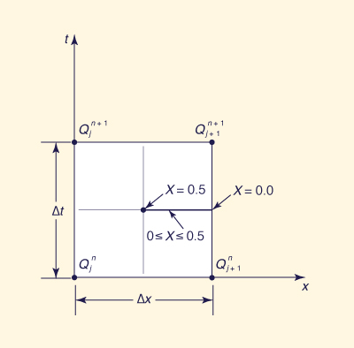
The discretization of Eq. 1 on the x-t plane (Fig. 1) leads to
(Ponce, 2014 b):
X (Q j n+1 - Q j n ) + (1 - X) (Q j+1n+1 - Q j+1 n ) (Q j+1 n - Q j n ) + (Q j+1n+1 - Q
j n+1 )
________________________________________________ + c _______________________________________ = 0
Δt 2 Δx
| (2) |
Fig. 1 Space-time discretization of the kinematic wave equation
following the Muskingum-Cunge method.
Simplifying Eq. 2:
|
X (Q j n+1 - Q j n ) + (1 - X) (Q j+1n+1 - Q j+1 n ) + 0.5 C [ (Q j+1 n - Q j n ) + (Q j+1n+1 - Q
j n+1 ) ] = 0
| (3) |
in which C = Courant number, defined as follows:
The solution of Eq. 3 is postulated in the following exponential form
(O'Brien et al., 1950;
Cunge, 1969):
|
Q = Q* e i (σx - βt )
| (5) |
in which σ = (2π /L) is the wavenumber, L is the wavelength of the disturbance, and β = (2 π /T )
is the wave period (Ponce and Simons, 1977).
4. CONVERGENCE RATIOS
The derivation of the convergence ratios has been described in detail
by Ponce and Vuppalapati (2016).
The convergence ratio with regard to wave amplitude is:
[(P - M)2 + N 2]1/2
R1 = ____________________
P
| (6) |
in which:
|
P = 1 - 2 (1 - p)(1 - S) S
| (6a) |
wherein
and C = Courant number (Eq. 4).
The convergence ratio with regard to wave phase is:
1 N
R2 = _________ tan-1 ( ________ )
C σΔx P - M
| (7) |
Therefore, given: (1)
weighting factor X (in Eq. 2), (2) spatial resolution L/Δx [from which σΔx
= (2π /L)Δx = 2π /(L/Δx)],
and (3) Courant number C (Eq. 4),
Eqs. 6 and 7 enable the calculation of the Muskingum-Cunge amplitude and phase
convergence ratios, respectively.
The calculation of the convergence ratios is accomplished
using the calculator
Online Muskingum-Cunge Convergence Ratios.
5. AMPLITUDE AND PHASE PORTRAITS
The plotting of convergence ratios R1 and
R2 as a function of Courant number C (in the abscissas)
and spatial resolution L/Δx (as the curve parameter)
leads to a set of amplitude and phase portraits R1 and R2,
respectively, a pair for each value of
weighting factor X in the range 0.0 ≤ X ≤ 0.5.
We observe that this range of analysis for the weighting factor X
is amply justified by kinematic wave theory
(Ponce et al., 1979 a).
Figures 2 to 8 show the amplitude and phase portraits of the Muskingum-Cunge method (Eq. 3),
for the following conditions: (a) Courant number
0.1 ≤ C ≤ 4.0, (b) spatial resolution 20 ≤ L/Δx ≤ 100,
shown at intervals of L/Δx = 20,
and (c) weighting factor 0.0 ≤ X ≤ 0.6, shown at intervals of X = 0.1 (7 × 2 = 14 graphs).
Note that the value X = 0.6 (Fig. 8) is included here only for comparison purposes, i.e.,
to show the numerical effect of
a value X > 0.5, which results in numerical amplification, R > 1; see Fig. 8 (a).
The selected range of Courant numbers shown (0.1 ≤ C ≤ 4.0) encompasses the central value C = 1, for which
absolute accuracy is obtained for X = 0.5; see Figs. 7 (a) for amplitude portrait and 7 (b) for phase portrait.
The range of spatial resolution shown in Figures 2 to 8 (20 ≤ L/Δx ≤ 100)
depicts five (5) values, varying from low (L/Δx = 20; poor resolution) to high
(L/Δx = 100; very good resolution). The spatial resolution is the
number of discrete intervals Δx
per wavelength L.
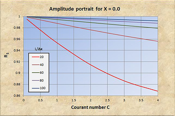
Fig. 2 (a) Amplitude portrait for X = 0.
|
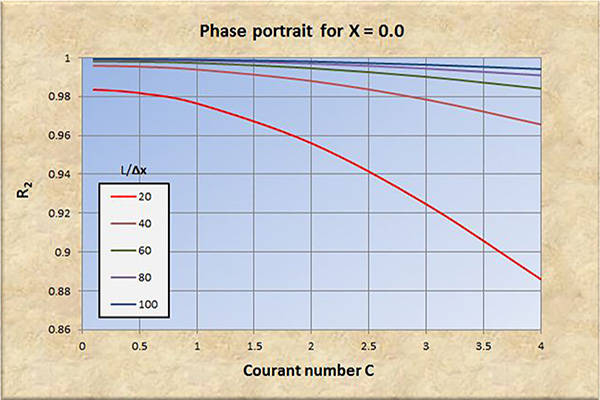
Fig. 2 (b) Phase portrait for X = 0.
|
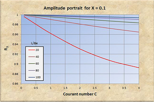
Fig. 3 (a) Amplitude portrait for X = 0.1.
|
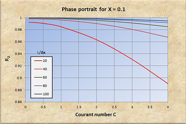
Fig. 3 (b) Phase portrait for X = 0.1.
|
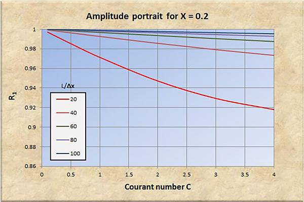
Fig. 4 (a) Amplitude portrait for X = 0.2.
|
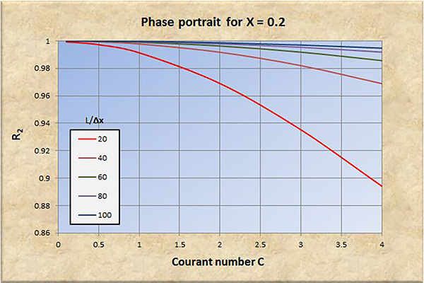
Fig. 4 (b) Phase portrait for X = 0.2.
|
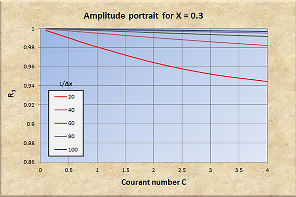
Fig. 5 (a) Amplitude portrait for X = 0.3.
|

Fig. 5 (b) Phase portrait for X = 0.3.
|
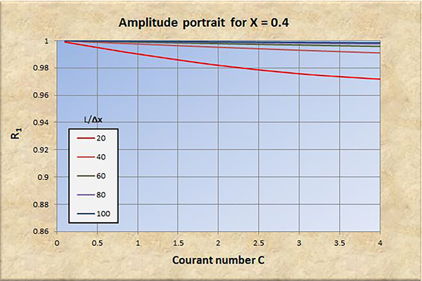
Fig. 6 (a) Amplitude portrait for X = 0.4.
|
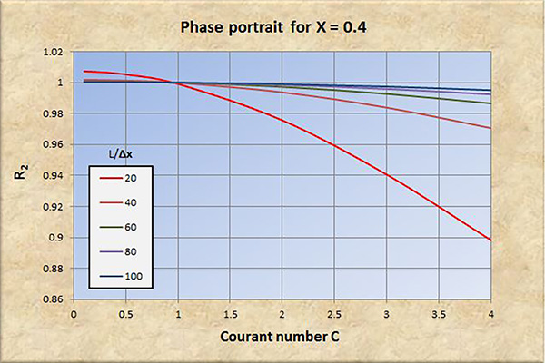
Fig. 6 (b) Phase portrait for X = 0.4.
|
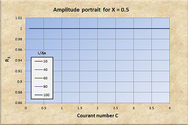
Fig. 7 (a) Amplitude portrait for X = 0.5.
|
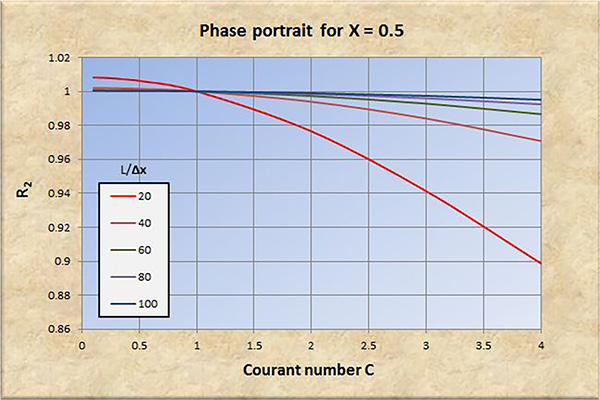
Fig. 7 (b) Phase portrait for X = 0.5.
|
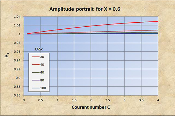
Fig. 8 (a) Amplitude portrait for X = 0.6.
|

Fig. 8 (b) Phase portrait for X = 0.6.
|
6. ANALYSIS
The examination of Figs. 2 to 8 leads to the following conclusions:
Perfect convergence amounts to R1 = 1 and
R2 = 1, i.e., implying that Eq. 2 is the exact solution of Eq. 1. It is
achieved only for X = 0.5 [confirm with Fig. 7 (a)]
and Courant number C = 1 [confirm with Fig. 7 (b)].
This behavior is due to the following reasons: (1) for X = 0.5, the numerical scheme (Eq. 2)
is fully centered (Fig. 1) and, therefore,
the second-order error
vanishes; and (2) for C = 1, the third-order error also vanishes
(Ponce et al., 1979 b).
For any X-C pair other than X = 0.5 and C = 1,
the numerical solution of Eq. 2 is only an approximation of the analytical solution of Eq. 1.
The accuracy of the approximation is a function of the following parameters: (a) spatial resolution
L/Δx;
(b)
Courant number C; and weighting factor X of the numerical scheme (Fig. 1).
As expected, convergence in both amplitude and phase
improves with an increase in spatial resolution. In Figures 2 to 8,
the low resolution (L/Δx = 20) is depicted in red color, while the high resolution
is shown in black. In particular, note the marked departure of the red-colored curves from the X-axis
(R = 1),
indicating a substantial lack of convergence for the low resolution case.
Convergence in both amplitude and phase degrades
with an increase in Courant number as C increases above 1, particularly as C ≫ 1; for example, for C = 4.
Convergence in amplitude improves substantially with an increase
of X in the range 0 ≤ X < 0.5. At X = 0.5, amplitude convergence is perfect for all
Courant numbers [see Fig. 7 (a)].
Convergence in phase improves slightly with an increase of X in the range 0 ≤ X < 0.5.
At X = 0.5, phase convergence is perfect only for C = 1 [see Fig. 7 (b)].
At low spatial resolutions,
refer to red curves in Figs. 2 (b) to 8 (b),
convergence in phase (as depicted by R2) degrades significantly
as Courant numbers decrease below C = 1, leading to R2 > 1, i.e., numerical instability [see Figs. 5 (b),
6 (b), y 7(b)].
For X > 0.5, as shown in Figs. 8(a) and 8(b), i.e., outside
of the
feasible range of X in Muskingum-Cunge routing,
the amplitude convergence
ratio R1 becomes positive (amplification) and, accordingly,
stability and convergence degrade in an explosive manner.
We conclude that the Muskingum-Cunge numerical model is a good representation of the analytical prototype, provided:
The spatial resolution L/Δx is sufficiently high,
preferably of the order of
L/Δx ≅ 100.
The Courant number C is sufficiently close to 1.
The weighting factor X is high enough in the range 0.0 ≤ X < 0.5;
preferably between 0.3 and 0.5.
Based on the analysis presented herein,
the recommended parameter values for reasonably adequate convergence are the following: (a) spatial resolution L/Δx ≅ 100; (b) Courant number C ≅ 1; and (c)
weighting factor X between 0.3 and 0.5.
7. APPLICATIONS
In practice, the convergence of the Muskingum-Cunge method depends on the values of Courant and cell Reynolds numbers, which in turn
depend on the hydraulics of the flow and the chosen grid size (Δx
and Δt)
(Ponce, 2014 b).
A set of amplitude and phase convergence ratios may be calculated
in terms of hydraulic and hydrologic variables.
To this end, define the time-of-rise tr of the flood wave as the time it takes it to reach the peak flow.
Assuming a sinusoidal perturbation as a first approximation, the time base, or wave period T is:
The wave celerity c is:
in which u is the mean flow velocity.
In turbulent
open-channel flow, the value of β
varies from β = 5/3 for a hydraulically wide channel, down to β = 1 for
an inherently stable channel (Ponce and Porras, 1995;
Ponce, 2014 c). For a rectangular channel, β may be approximated as 5/3, for a triangular channel
as 4/3, and for a hydraulically wide natural channel, a reasonably good approximation
is β = 1.6.
The wavelength L of the perturbation is:
The unit-width discharge q is:
in which d is the mean flow depth. The spatial resolution is L/Δx.
The Courant number (Eq. 4), repeated here for convenience with a new equation number, is:
The cell Reynolds number is
(Ponce, 2014e):
q
D = ___________
So c Δx
| (13) |
By definition, the Muskingum-Cunge weighting factor X is:
1
X = ____ (1 - D)
2
| (14) |
For a given case, Eqs. 6 and 7, with support from Eqs. 8 to 14, enable the calculation
of the convergence ratios of the Muskingum-Cunge method.
Two cases are explained here: (1) theoretical, and (2) practical.
The calculation of the theoretical Muskingum-Cunge convergence ratios may be accomplished
using the calculator
Online Muskingum-Cunge Convergence Ratios. Three
examples are discussed here: (A) perfect convergence, (B) good convergence, and
(C) poor convergence. For Case A, assume X = 0.5; L /Δx = 100; and C = 1.
The results, shown in Fig. 9, are: R1 = 1, and R2 = 1,
confirming the perfect convergence of the Muskingum-Cunge method for the case of X = 0.5, L /Δx = 100,
and C = 1.
Fig. 9 Muskingum-Cunge convergence ratios
for X = 0.5, L /Δx = 100, and C = 1: R1 = 1;
R2 = 1.
For Case B, assume X = 0.35; L /Δx = 60; and C = 1.1.
The results, shown in Fig. 10, are: R1 = 0.998195; R2 = 0.999563,
confirming the good convergence of the Muskingum-Cunge method for the case of X = 0.35,
L /Δx = 60,
and C = 1.1.
Fig. 10 Muskingum-Cunge convergence ratios
for X = 0.35, L /Δx = 60, and C = 1.1: R1 = 0.998185; R2 = 0.999563.
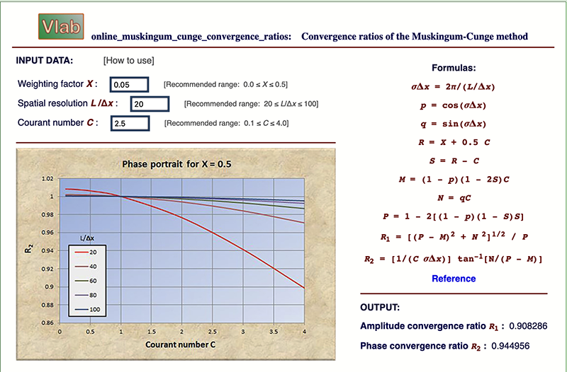
For Case C, assume X = 0.05; L /Δx = 20; and C = 2.5.
The results, shown in Fig. 11, are: R1 = 0.908286; R2 = 0.944956,
confirming the poor convergence (i.e., R ratios much smaller than 1) of the Muskingum-Cunge method for the case of X = 0.05,
L /Δx = 20,
and C = 2.5.
Fig. 11 Muskingum-Cunge convergence ratios
for X = 0.05, L /Δx = 20, and C = 2.5:
R1 = 0.908286;
R2 = 0.944956.
The calculation of the practical Muskingum-Cunge convergence ratios may be accomplished
using the calculator
Online Muskingum-Cunge Convergence Ratios Practical. Two
examples are discussed here: (D) small stream, and
(E) large stream.
For Example D, assume the following data set:
Mean velocity u = 1.75 m/s;
Mean flow depth d = 2.3 m;
Mean channel slope S = 0.0013;
Rating exponent β = 1.6;
Flood wave time-of-rise tr = 24 hr;
Reach length Δx = 4800 m; and
Time interval Δt = 0.5 hr.
The application of
Online Muskingum-Cunge Convergence Ratios Practical, shown in Fig. 12, leads to:
R1 = 0.99953;
R2 = 0.999915.
In this case, the spatial resolution is L/Δx = 100.8; the Courant number is C = 1.05; and the weighting factor is X =
0.385. All three parameters are confirmed to lie within the recommended ranges for adequate convergence.
Fig. 12 Muskingum-Cunge convergence ratios
for Example D: R1 = 0.99953;
R2 = 0.999915.
For the next, and last, example E, assume the following data set:
Mean velocity u = 0.5 m/s;
Mean flow depth d = 6.2 m;
Mean channel slope S = 0.018;
Rating exponent β = 1.65;
Flood wave time-of-rise tr = 36 hr;
Reach length Δx = 2500 m; and
Time interval Δt = 1.5 hr.
The application of
Online Muskingum-Cunge Convergence Ratios Practical, shown in Fig. 13, leads to:
R1 = 0.9996;
R2 = 0.999014.
In this case, the spatial resolution is L/Δx = 85.536; the Courant number is C = 1.728; and the weighting factor is X =
0.458. All three parameters are confirmed to lie within the recommended ranges for adequate convergence.
Fig. 13 Muskingum-Cunge convergence ratios
for Example E: R1 = 0.9996;
R2 = 0.999014.
8. CONCLUDING REMARKS
Herein
we endeavor to clarify some of the concepts elaborated in this article, with aim to encourage its wider use.
On the Courant number.
Numerical convergence, which may be taken as
numerical accuracy, depends on spatial resolution L/Δx and temporal resolution T/Δt, both of these
being dimensionless expressions of grid size. In computacional hydraulics, the Courant number C is
defined as
the ratio of physical celerity to grid "celerity": C =
c / (Δx /Δt) = c (Δt /Δx) = (L/T) (Δt /Δx)
= (L/Δx) / (T/Δt). In other words, the Courant number is indeed
the ratio of spatial to
temporal resolution. Only two of the three variables: (1) spatial resolution, (2) temporal resolution, and (3)
Courant number,
are required to fully define the analysis. As stated in Section 2 of this article,
we use spatial resolution and Courant number, as shown in Figs. 2 to 8.
On the limitations of the Muskingum method. The classical
Muskingum method of flood routing (Chow, 1959) solves the kinematic wave
equation numerically, thus, introducing a certain undefined
amount ot numerical diffusion. In practice, the latter manifests itself as an appreciable amount of
attenuation, or diffusion, of the flood wave being calculated. There is no relation of this introduced
numerical diffusion with the
true physical diffusion, if any, of the problem under consideration [Note: Recall that the true solution of a kinematic wave
does not allow for any physical diffusion]. Therefore, the classical Muskingum method fails to solve the flood propagation problem
in a meaningful way. The actual solution will be heavily dependent on the chosen grid size,
which has not been explicitly related
to the physical problem at hand.
On the strength of the Muskingum-Cunge method. Unlike the Muskingum method, the Muskingum-Cunge method
(M-C method) is physically and numerically based. The weighting factor X is calculated by Eq. 14, which in turn is based on physical and numerical variables (Eq. 13).
This remarkable feature of the M-C method is unique in the field of computational hydraulics, enabling it to become
grid independent through a wide range of values of spatial resolution. Once the spatial grid
interval Δx is selected or determined a priori, the weighting factor X is fixed
by Eq. 14. In this way, the values of physical and numerical diffusion have been matched, and this procedure
renders the
method and its result grid independent!
On the meaning of the amplitude and phase portraits. Since the kinematic wave equation (Eq. 1)
exhibits no physical diffusion (i.e., damping), Eq. 6 (amplitude portrait) is a measure of the numerical diffusion (i.e., a value less than 1)
or, alternatively, numerical
amplification (i.e., negative diffusion, a value greater than 1), after one time increment Δt
(Ponce et al., 1979 d).
Correspondingly,
a similar conclusion for wave phase (either retardation or acceleration) follows from Eq. 7 (phase portrait).
It should not escape our attention that the closeness to 1 of both portrait values shown in Figs. 9 to 13
reflects the fact
that the values are applicable per time increment Δt.
9. SUMMARY
A comprehensive review of the Muskingum-Cunge method's amplitude and phase portraits is accomplished.
Expressions for the
amplitude convergence ratio R1 and phase convergence ratio R2 are expressed as a function
of the following basic numerical parameters:
(a) spatial resolution L /Δx; (b) Courant number C; and (c) weighting factor X.
An online calculator
Online Muskingum-Cunge Convergence Ratios is used for convenience.
For practical applications, input may be expresssed in terms of
relevant hydraulic variables, such as mean velocity, flow depth, channel slope, rating exponent,
and flood wave time-of-rise. For this case, an online calculator
Online Muskingum-Cunge Convergence Ratios Practical is developed.
REFERENCES
Chow, V. T. 1959. Open-channel hydraulics. McGraw-Hill, New York.
Cunge, J. A.. 1969.
On the subject of a flood propagation computation method (Muskingum method). Journal of Hydraulic Research, Vol. 7, No. 2, 205-230.
Hayami, S. 1951. On the propagation of flood waves. Bulletin No. 1, Disaster Prevention Research Institute,
Kyoto University, Kyoto, Japan, December.
Koussis, A. 1978. Theoretical estimation of flood routing parameters. Journal of the Hydraulics Division, ASCE,
Vol. 104, No. HY1, Proc. Paper 13456, January, 109-115.
Leendertse, J. J. 1967. Aspects of a computational model for long-period water wave propagation. Report RM-5294-PR, The Rand Corporation,
Santa Monica, California, May.
McCarthy, G. T. 1938. The unit hydrograph and flood routing. Unpublished manuscript, presented at a conference of the North Atlantic Division,
U.S. Army Corps of Engineers, June 24, 1938.
Natural Environment Research Council. 1975. Flood Studies Report, Vol. III: Flood Routing Studies, London, England.
O'Brien, G. G., M. A. Hyman, and S. Kaplan. 1950. A study of the numerical solution of partial differential equations.
Journal of Mathematics
and Physics, Vol. 29, No. 4, 223-251.
Ponce, V. M. and D. B. Simons. 1977. Shallow wave propagation in open channel flow.
Journal of the Hydraulics Division, ASCE, Vol. 103, No. HY12, December, 1461-1476.
Ponce, V. M. and V. Yevjevich. 1978.
Muskingum-Cunge method with variable parameters.
Journal of the Hydraulics Division, ASCE, Vol. 104, No. HY12, December, 1663-1667.
Ponce, V. M., Y. H. Chen, and D. B. Simons. 1979. Unconditional stability in convection computations. Journal of the Hydraulics Division, ASCE, Vol. 105, No. HY9, September, 1079-1086.
Ponce, V. M. 1986. Diffusion wave modeling
of catchment dynamics.
Journal of Hydraulic Engineering, ASCE, Vol. 112, No. 8, August, 716-727.
Ponce, V. M. and P. J. Porras. 1995. Effect of cross-sectional shape on free-surface instability. Journal of Hydraulic Engineering, ASCE, Vol. 121, No. 4,
April, 376-380.
Ponce, V. M. 2014. Fundamentals of open-channel hydraulics.
Online text.
Ponce, V. M. and B. Vuppalapati. 2016.
Muskingum-Cunge amplitude and phase portraits
with online computation.
Online article.
|