The Courant number, Computational Hydraulics, Victor M. Ponce

Flood stage on the Chané river, Santa Cruz department, Bolivia (January 1990).

THE COURANT NUMBER

Victor M. Ponce

Professor Emeritus of Civil and Environmental Engineering

San Diego State University, San Diego, California

14 December 2023

ABSTRACT. In this paper we focus on the role of the Courant number in computational hydraulics, particularly in the modeling of the pure convection problem. We throw a renewed light onto the properties of stability and convergence of a class of popular explicit linear numerical schemes of the pure convection equation. Both conditional and unconditional stability are shown to be possible with explicit schemes. In addition, the existence of numerical diffusion, ostensibly due to the first-order errors of the numerical scheme, is shown to affect the computation, rendering the solution grid-dependent and distinctively diffusive for all cases other than Courant number C = 1.

1. INTRODUCTION

The Courant number is a fundamental concept in the field of Computational Fluid Dynamics (CFD) and, by extension, in Computational Hydraulics. The number effectively connects the physical and numerical properties of a computational scheme, with specific application to the convection problem, in other words, the well-known advection of fluid mechanics. The Courant number is defined as the ratio of a physical velocity u to the grid velocity Δx /Δt. In practice, the Courant number is commonly expressed in the following form: C = u Δt /Δx (Ponce, 2014).

The name Courant recognizes the life work of Richard Courant, a renowned German-American mathematician and early contributor to the field of applied mathematics. The concept of Courant number is rooted in the pioneering Courant-Friedrichs-Lewy condition, which is widely referred to as the CFL condition (Courant et al., 1928).

In this article, we endeavor to perform a contemporary analysis of the Courant number, throwing renewed light onto its behavior. We focus specifically on the numerical solution of the convection problem, unveiling properties that may have been hitherto hidden in conventional applications of computational fluid dynamics and hydraulics.

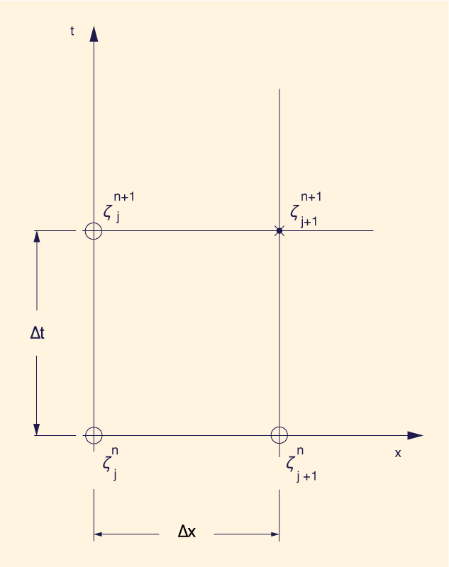
2. THE CONVECTION PROBLEM AND THE FOUR-POINT GENERAL SCHEME

In order to set the stage for the analysis that will follow, we begin by conceptualizing the convection problem of fluid mechanics. A physical quantity ζ will move, in space x and time t, with a certain convective velocity u following a first-order partial differential equation of the following form (Ponce et al., 1979):

      ∂ζ              ∂ζ
   ^_____ + u ^_____ = 0
      ∂t              ∂x           (1)

This equation may be solved numerically in various ways. A conveniently general explicit linear finite difference formulation is the following four-point scheme (Fig. 1):

X (ζ_jⁿ⁺¹ - ζ _jⁿ) + (1-X) (ζ_j+1ⁿ⁺¹ - ζ_j+1ⁿ) Y (ζ_j+1ⁿ - ζ_jⁿ) + (1-Y)(ζ_j+1ⁿ⁺¹ - ζ_jⁿ⁺¹)
[ ^{_____________________________________}] + u [^{_____________________________________}] = 0
Δt Δx

(2)

Fig. 1 Discretization of the convection equation (Eq. 1) following Eq. 2.

In Equation 2, solving for the unknown value ζ_j+1ⁿ⁺¹ leads to the following routing equation:

ζ_j+1ⁿ⁺¹ = C₁ ζ_jⁿ + C₂ ζ_jⁿ⁺¹ + C₃ ζ_j+1ⁿ

(3)

The routing coefficients are defined as follows:

                     (X + CY)
C₁ = ^{_____________________}
             (1 + C) - (X + CY) (4)

                C - (X + CY)
C₂ = ^{____________________}
            (1 + C) - (X + CY) (5)

                1 - (X + CY)
C₃ = ^{____________________}
            (1 + C) - (X + CY) (6)

in which C is the Courant number defined as follows:

Δt
C = u ^_____
Δx (7)

For a given Courant number, with the weighting factors X and Y having been established beforehand, and using Eqs. 2 to 7, the computation proceeds to calculate the values of ζ for each and every one of the specified grid points in the computational domain.

Equation 3, with its supporting equations 4-7, constitutes a family of numerical schemes of the convection equation, Eq. 1. Their stability and convergence properties depend on the values of X, Y, and C. The first two, referred to as weighting factors, and C, the Courant number, uniquely characterize the chosen scheme. Ostensibly, the Courant number is the ratio of the convective velocity u to the grid ratio or "grid velocity" Δx /Δt.

3. NUMERICAL DIFFUSION AND DISPERSION

Equation 1 describes convection, a first-order process; therefore, diffusivity, a second-order process, and dispersivity, a third-order process, are not accounted for (Ponce, 2023). However, Eq. 2, a numerical solution of Eq. 1 will typically show a diffusive and/or a dispersive behavior due to the finite grid size. This is attributed to numerical diffusion (the error of the first-order term of the scheme) and numerical dispersion (the error of the second-order term).

A measure of the amount of numerical diffusion and dispersion may be obtained from the approximation error of the finite difference scheme, Eq. 2. This error may be obtained by expanding the grid function ζ(jΔx, nΔt) in Taylor series about point (jΔx, nΔt), leading to (Cunge, 1969; Ponce et al., 1979):

                     1                      1             ∂² ζ
R = u Δx [( ^____ - X ) + C (^____ - Y )]^_____
                     2                      2              ∂x²

                                1                        1                    ∂³ ζ
+ u Δx² { (1 - C ) [ ^____ ( X + CY) - ^____ (1 + C ) ] } ^_____ + ο(Δx³)
                                2                        3                      ∂x³ (8)

in which R = the approximation error. From Eq. 8, we note that for X = Y = 1/2, the scheme is of second-order accuracy. i.e., R = ο(Δx²). Furthermore, for C = 1, the accuracy is of third order; that is, the numerical dispersion vanishes. In point of fact, for X = Y = 1/2 and C = 1, the exact solution of the convection equation (Eq. 1) is obtained.

In Equation 8, the coefficient of the second-order term ∂²ζ /∂x² is referred to as the numerical diffusion coefficient and defined as follows:

1 1
μ_n = u Δx [(^____ - X ) + C (^____ - Y )]
2 2 (9)

Positive values of μ_n cause the scheme to diffuse numerically; negative values to amplify numerically. While in the former convergence is impaired, in the latter stability suffers. Both stability and convergence improve as μ_n → 0. Table 1 summarizes the stability and convergence properties of three common first-order schemes.

Table 1. Numerical properties of three common first-order explicit linear schemes (Eq. 2) of the pure convection equation (Eq. 1).
Scheme description	X	Y	*μ_n*	Courant stability condition	Convergence (μ_n → 0)
(1)	(2)	(3)	(4)	(5)	(6)
I. Forward-in-time, backward-in-space	0	1	(1/2) u Δx (1 - C)	C ≤ 1	C → 1
II. Forward-in-space, backward-in-time,	1	0	(1/2) u Δx (C - 1)	C ≥ 1	C → 1
III. Backward-in-time, backward-in-space	0	0	(1/2) u Δx (1 + C)	All C	No C

I. Forward-in-time, backward-in-space scheme features.

The forward-in-time, backward-in-space scheme is centered around node ζ_j+1ⁿ in Fig. 1.
The temporal derivative is taken on the right side of the square box and the spatial derivative along the bottom.
The numerical diffusion coefficient is: μ_n = (1/2) u Δx (1 - C).
The scheme is stable for C ≤ 1 and unstable for C > 1.
The scheme converges to the analytical solution (of the convection equation Eq. 1) as C → 1 (from the left).
The more refined the grid size (as Δx ↠ 0), the faster is the rate of convergence.
The scheme is conditionally stable, becoming unstable for C > 1.

II. Forward-in-space, backward-in-time scheme features.

The forward-in-space, backward-in-time numerical scheme is centered around node ζ_jⁿ⁺¹ in Fig. 1.
The temporal derivative is taken on the left side of the square box and the spatial derivative along the top.
The numerical diffusion coefficient is: μ_n = (1/2) u Δx (C - 1).
The scheme is stable for C ≥ 1 and unstable for C < 1.
The scheme converges to the analytical solution (of the convection equation Eq. 1) as C → 1 (from the right).
The more refined the grid size (Δx ↠ 0), the faster is the rate of convergence.
The scheme is conditionally stable, becoming unstable for C < 1.

III. Backward-in-space, backward-in-time scheme features.

The backward-in-space, backward-in-time scheme scheme is centered around node ζ_j+1ⁿ⁺¹ in Fig. 1.
The temporal derivative is taken on the right side of the square box and the spatial derivative along the top.
The numerical diffusion coefficient is: μ_n = (1/2) u Δx (1 + C).
The scheme is unconditionally stable, i.e., stable for any value of C.
However, this scheme does not converge to the analytical solution of the convection problem for any value of C, even as Δx → 0.

The present analysis enables the following conclusions:

Explicit schemes of the pure convection equation (Eq. 1), such as Eq. 2, may be either conditionally or unconditionally stable, depending on the way the scheme is formulated. Thus, the statement that all explicit schemes are subject to a stability condition is not correct.
Per force, since the grid size is always finite, explicit schemes such as that of Eq. 2 actually introduce varying amounts of numerical diffusion. Only for Courant number C = 1 the numerical diffusion vanishes; therefore, in this case the numerical solution of the scheme embodied by Eq. 2 is the true solution of the convection equation (Eq. 1).
In all other cases, i.e., specifically for C < 1 in the forward-in-time backward-in-space scheme, or C > 1 in the backward-in-time forward-in-space scheme, the numerical solution turns out to be effectively a diffusion wave, featuring varying amounts of numerical diffusion (Cunge, 1969; Ponce, 2023).

Contrary to explicit schemes, implicit schemes have been favored in the past due to their perceived improved stability properties, purportedly featuring what has often been referred to as "unconditional stability". Experience, however, points otherwise. In a general sense, both explicit and implicit numerical schemes are subject to issues of stability and convergence. An appropriate von Neumann analysis is recommended to substantially improve numerical modeling practice (Ponce et al., 1978).

4. SUMMARY

In this paper we focus on the role of the Courant number in computational hydraulics, particularly in the modeling of the pure convection problem. We throw a renewed light onto the properties of stability and convergence of a class of popular explicit linear numerical schemes of the pure convection equation. Both conditional and unconditional stability are shown to be possible with explicit schemes. In addition, the existence of numerical diffusion, ostensibly due to the first-order errors of the numerical scheme, is shown to affect the computation, rendering the solution grid-dependent and distinctively diffusive for all cases other than Courant number C = 1. The classical von Neumann analysis is recommended to improve modeling practice.

REFERENCES

Courant, R., K. Friedrichs, and H. Lewy. 1928. �ber die partiellen Differenzengleichungen der mathematischen Physik, Mathematische Annalen, vol. 100, p. 32-74.

Cunge, J. A. 1969. On the Subject of a Flood Propagation Computation Method (Muskingum Method). Journal of Hydraulic Research, Vol. 7, No. 2, 205-230.

Ponce, V. M., H. Indlekofer, and D. B. Simons. 1978. Convergence of four-point implicit water wave models. Journal of the Hydraulics Division, ASCE, Vol. 104, No. HY7, July, 947-958.

Ponce, V. M., Y. H. Chen, and D. B. Simons. 1979. Unconditional stability in convection computations. Journal of the Hydraulics Division, ASCE, Vol. 105, No. HY9, September, 1079-1086.

Ponce, V. M. 2014. Engineering Hydrology: Principles and Practices. Second edition, online.

Ponce, V. M. 2023. Is dispersion important in flood routing? Online paper.

Ponce, V. M. 2023. When is the diffusion wave applicable? Online paper.

231214