|
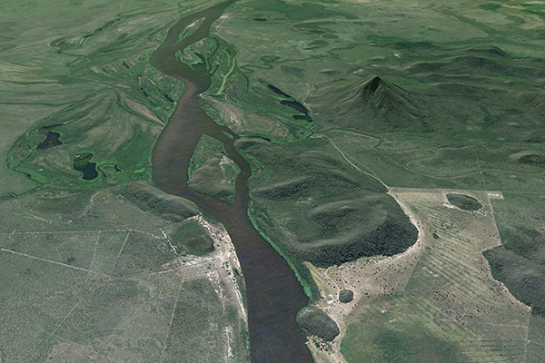
Fecho dos Morros, literally Closing of the Hills, a substantial tectonic uplift feature (≃ 40 m) IS THE DYNAMIC HYDRAULIC DIFFUSIVITY ALTOGETHER BETTER THAN ITS KINEMATIC COUNTERPART?
Professor of Civil and Environmental Engineering
San Diego State University, San Diego,
California
1. INTRODUCTION
Runoff diffusion
is the property of free-surface flows to diffuse appreciably, attenuating unsteady flow stages
in Nature's apparently determined quest
to return the flow to its steady uniform condition. Diffusion
is characterized by the coefficient of the second-order term of the partial differential
equation governing the flow
(Ponce, 2014a: Diffusion waves). This coefficient is commonly referred to as hydraulic diffusivity.
Since the 1950s, several mathematical expressions for hydraulic diffusivity have been developed
as more information became available.
Hayami (1951) developed the first expression for hydraulic diffusivity.
He was followed by Dooge (1973)
and later by Dooge and others (1982), culminating in the
work of Ponce (1991),
who identified the Vedernikov number in the expression for dynamic
hydraulic diffusivity.
The question remains as to whether the aforementioned improvements are indeed such when practical applications
are considered. This article reviews and compares Hayami's and Ponce's
expressions for hydraulic diffusivity.
In the process, we manage to advertently cast a doubt on the existential nature of dynamic waves
(Ponce, 2023a).
2. KINEMATIC HYDRAULIC DIFFUSIVITY
Hayami (1951) pioneered the diffusion wave approach with
free-surface flow (Ponce, 2023a) with the specific purpose for flood routing applications.
His approach has been widely referred to in the literature as
Hayami's diffusion analogy.
in which ν = hydraulic diffusivity, qo = reference
unit-width discharge, and So = bottom slope.
Since Hayami's formulation explicitly excludes inertia,
it is properly a kinematic hydraulic diffusivity, to follow the work of
Lighthill and Whitham (1955)
on kinematic wave theory. Therefore:
in which νk = kinematic hydraulic diffusivity.
3. DYNAMIC HYDRAULIC DIFFUSIVITY
Using linear theory,
Dooge (1973) derived the complete
convection-diffusion equation
of flood flows, including the inertia terms, leading to the formulation of a dynamic
hydraulic diffusivity:
in which νd = dynamic hydraulic diffusivity.
In Equation 3, F = Froude number of the equilibrium flow, defined as follows:
Dooge and others (1982) improved the original Dooge
formulation (Eq. 3) by expressing the fraction within parenthesis in terms
of the exponent β of the discharge-flow area rating
In fact, for Chezy friction in a hydraulically wide channel, β = 1.5.
Therefore, for this case, Eq. 4 is shown to be equivalent to
Ponce (1991a; 1991b) recognized
the term (β - 1)F in Eq. 4 as the Vedernikov number V
(Ponce, 2014b),
thereby reducing the
expression for dynamic hydraulic diffusivity to the following:
We note that while the kinematic
hydraulic diffusivity (Eq. 2) is independent
of the Vedernikov number, the dynamic
hydraulic diffusivity (Eq. 5)
has a clearly defined threshold for V = 1, being positive for
4. TYPES OF WAVES IN OPEN-CHANNEL FLOW
While
Equation 2 does not include the inertia terms,
Equation 5 clearly does. Therefore,
Eq. 5 should be a more accurate description of hydraulic diffusivity. To throw additional light on the issue,
Table 1 shows the various types of waves in unsteady open-channel flow, including classical and common names.
Equation 2 was derived
by Hayami by neglecting inertia in the equation of motion (Table 1, Line 2),
i.e., a kinematic wave with diffusion; therefore, we confirm the appropriateness of the name kinematic hydraulic diffusivity.
On the other hand, Eq. 5 was derived by considering all terms in the equation of motion (Table 1, Line 4),
i.e., a mixed kinematic-dynamic wave,
commonly referred to as a dynamic wave; therefore, the name dynamic hydraulic diffusivity appears justified
at this juncture.
We have confirmed that Eq. 2 is an approximation for hydraulic diffusivity and that Eq. 5 is the complete expression. The question arises as to what is the actual difference between the two formulations when practical applications are considered. In the following section (Section 5) we evaluate the difference between the two alternative formulations for hydraulic diffusivity (Eqs. 2 and 5) using a catchment model of overland flow.
5. COMPARISON BETWEEN DIFFUSIVITIES
In this section, we use an overland flow
model to test the difference between the two formulations of hydraulic diffusivity,
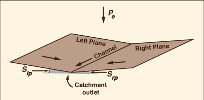
Eqs. 2 and 5. The model simulates catchment dynamics using an open-book
geometric configuration,
i.e., two planes (left and right) and one channel in the middle (Fig. 1)
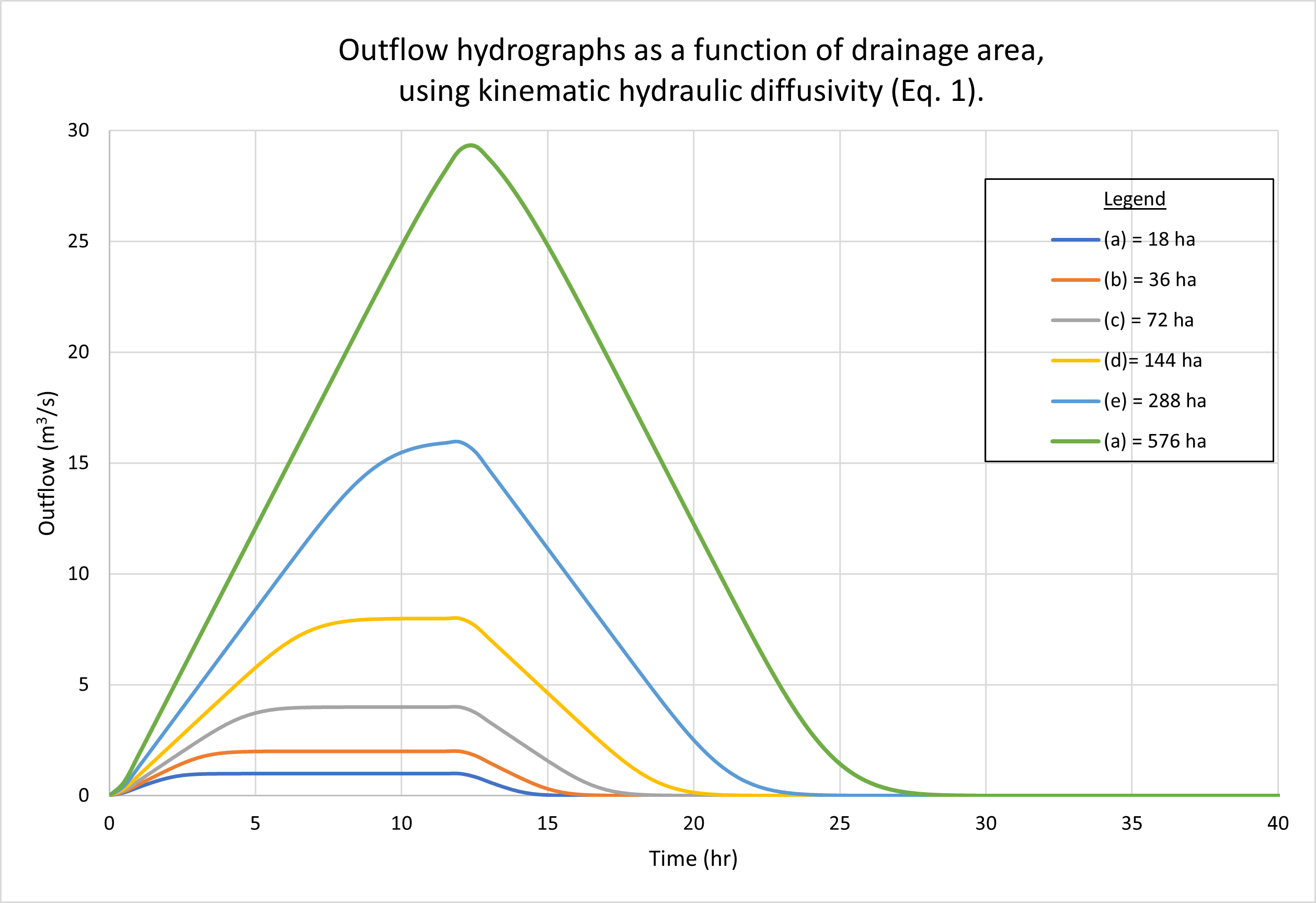
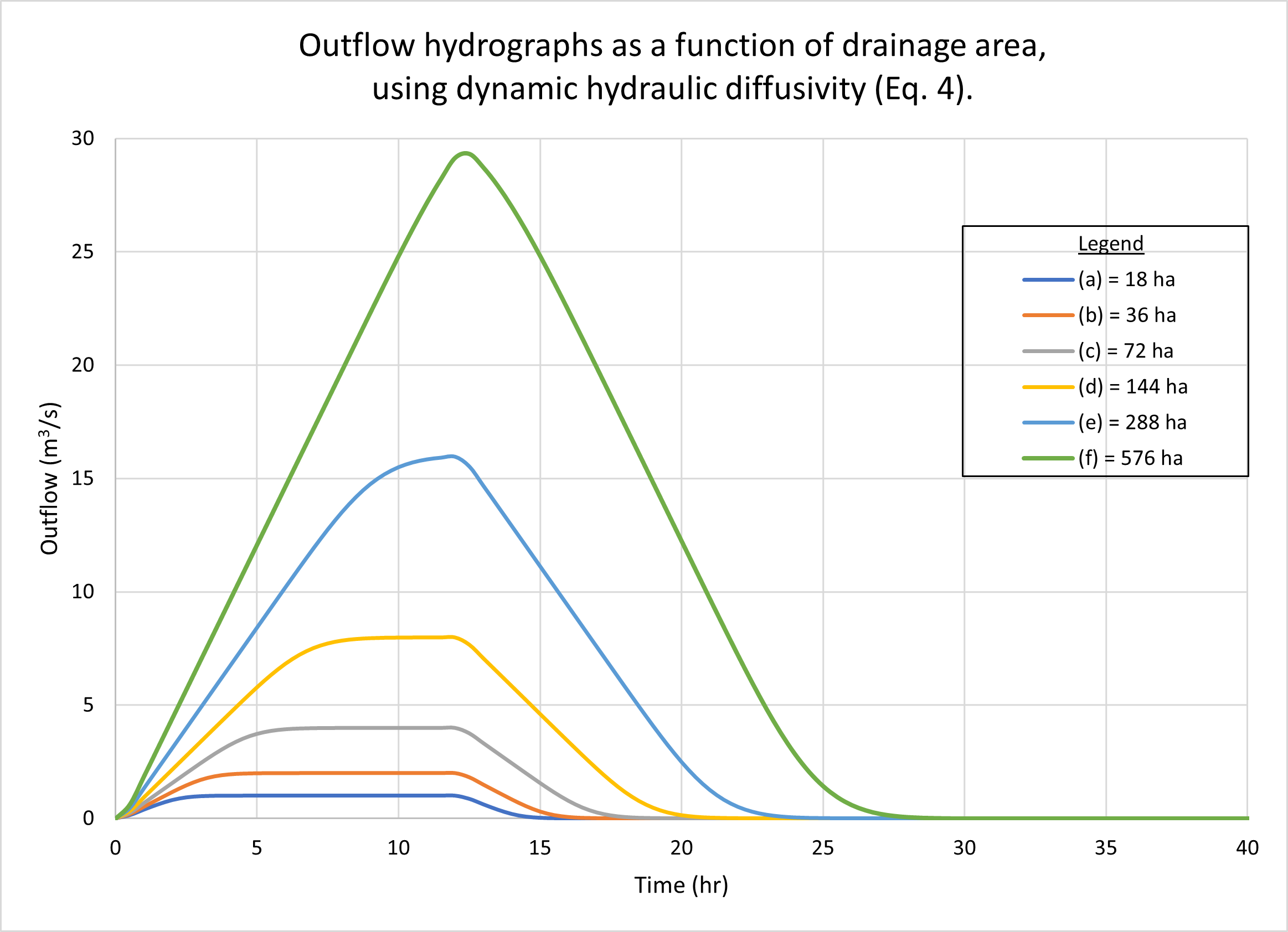
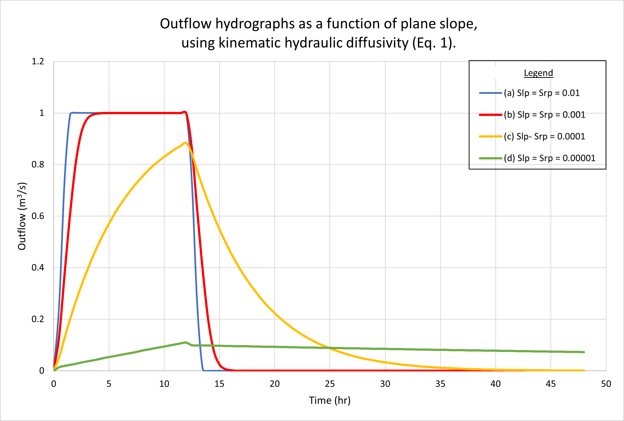
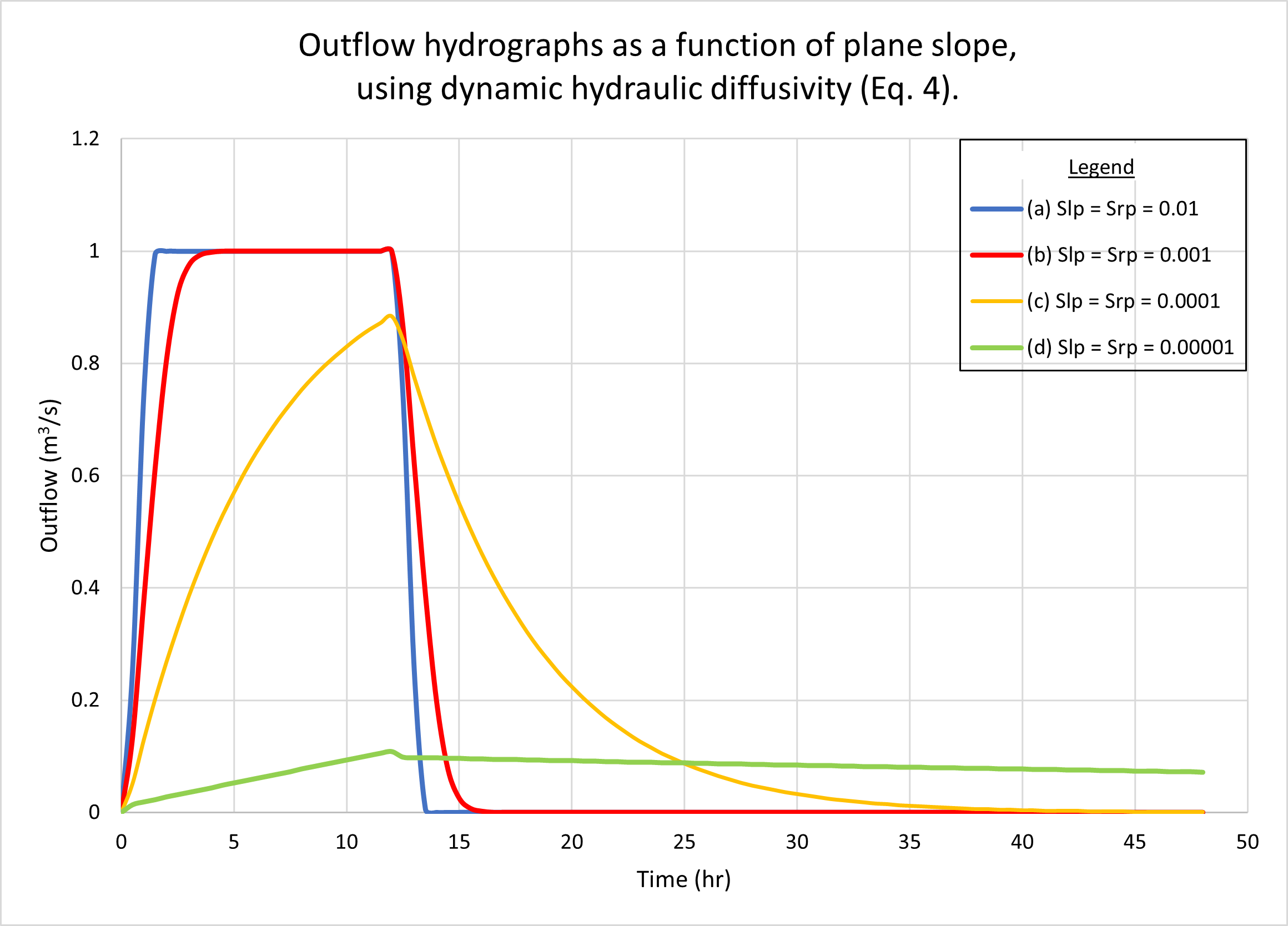
The results show negligible differences between the two diffusivities under a wide range of flow conditions. Kinematic waves (Table 1, Line 1) and diffusion waves (Table 1, Line 2) were used in the tests because these were the only ones likely to be encountered in actual practice. The Vedernikov number in the planes was quite low, around 0.03. Figure 2 shows the outflow hydrographs for drainage areas varying from 18 hectares (small) to 576 hectares (midsize). Figure 3 shows the outflow hydrographs for plane slopes (left and right) varying from 0.01 (steep) to 0.00001 (mild). No appreciable differences are observed between hydrographs generated using kinematic [(a) figures] and dynamic [(b) figures] hydraulic diffusivities.
The lack of any appreciable difference between output hydrographs when comparing
results using kinematic and dynamic diffusivities (Eqs. 2 and 5) is attributed to the
type of modeling used in this study.
The examples shown in Figs 2 and 3 depict kinematic waves (Table 1, Line 1) and diffusion waves (Table 1, Line 2), since these are the ones likely to be encountered in actual practice. By definition, these waves are not subject to substantial diffusion; thus, featuring relative small values of either of the two diffusivities. We conclude that when modeling catchment flows using kinematic and diffusion waves, the difference between hydraulic diffusivities is likely to be negligible.
6. DOES THE DYNAMIC WAVE REALLY EXIST IN PRACTICE?
A question to be addressed at this juncture is
the nature of mixed kinematic-dynamic waves
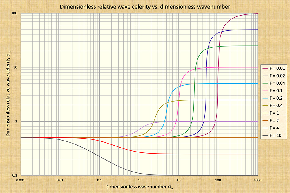
Further confirmation of the correctness of Lighthill and Whitham's observations regarding the strong dissipative nature of dynamic waves was given by Ponce and Simons (1977), who used linear stability analysis to derive celerity and attenuation functions for the four types of shallow-water waves shown in Table 1. Ponce and Simons (1977) identified the dimensionless wavenumber σ* as the fundamental physical parameter describing the propagation of shallow-water waves. Their findings are summarized in Fig. 4.
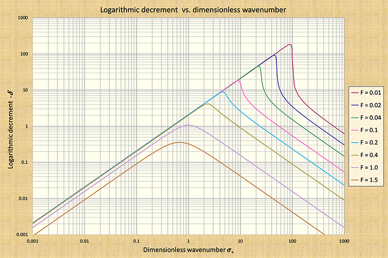
The findings of Ponce and Simons (1977) confirm the very strong dissipative tendencies of mixed kinematic-dynamic waves, commonly referred to in the hydraulic engineering literature simply as "dynamic waves" (Fread, 1985). The peak attenuation amount occurs at the point of inflection in the dimensionless relative celerity cr* vs dimensionless wavenumber σ* [compare Fig. 4 (a) with Fig. 4 (b)]. Note that the amount of wave attenuation increases markedly with a decrease in equilibrium flow Froude number. For the lowest Froude number shown in Fig. 4, F = 0.01, the peak logarithmic decrement is δ = 180, corresponding to σ* = 90 [Fig. 4 (b)].
Table 2 shows peak logarithmic decrements (Column 3) for
the range of subcritical Froude numbers between
Having demonstrated that the mixed kinematic-dynamic wave may not be there for us,
we still have a choice of using or not the dynamic hydraulic diffusivity
(Eq. 5) in all applications of unsteady free-surface flow,
including both catchment and channel flow.
7. SUMMARY
A comparison between
kinematic and dynamic hydraulic diffusivities using an actual catchment
model of overland flow is accomplished. The kinematic hydraulic diffusivity
is the well known Hayami diffusivity, which is independent of the Vedernikov number.
On the other hand, the dynamic hydraulic diffusivity is a function of the Vedernikov number.
Several examples of rainfall-runoff conversions using the catchment model
show that the difference between these two formulations of hydraulic
diffusivity is negligible. This may be attributed
to the very low Vedernikov numbers typically featured
in catchment models, or to the specification of kinematic and diffusion waves in the test
cases, since these waves are the only ones likely to be encountered in actual practice.
The question of the true nature of mixed kinematic-dynamic waves is examined using
available analytical data. It is concluded that given their extremely strong dissipative tendencies,
mixed waves may not be there for us to calculate. Nevertheless,
the dynamic hydraulic diffusivity is advocated
as the method of choice because it is the complete solution, it is
applicable to all types of routing, including catchment and channel flow,
and it does not significantly complicate the methodology.
REFERENCES
Dooge, J. C. I. 1973.
Linear theory of hydrologic systems: Lecture 9. Technical Bulletin No. 1468, U.S. Department of Agriculture, Washington, D.C.
Dooge (1973).
Dooge, J. C. I., W. B. Strupczewski, and J. J. Napiorkoswki. 1982. Hydrodynamic derivation of storage parameters in the Muskingum model.
Journal of Hydrology, 54, 371-387.
Fread, D. L. 1985. "Channel Routing," in Hydrological Forecasting,
M. G. Anderson and T. P. Burt, eds. New York: John Wiley.
Hayami, I. 1951.
On the propagation of flood waves. Bulletin, Disaster Prevention Research Institute,
No. 1, December.
Lighthill, M. J. and G. B. Whitham. 1955.
On kinematic waves. I. Flood movement in long rivers.
Proceedings,
Natural Resources Conservation Service (NRCS). 1985. National Engineering Handbook. Section 4: Hydrology, Washington, D.C.
(First edition: 1954).
Ponce, V. M. and D. B. Simons. 1977.
Shallow wave propagation in open channel flow.
Journal of Hydraulic Engineering, ASCE, 103(12), 1461-1476.
Ponce, V. M. 1986.
Diffusion wave modeling of catchment dynamics.
Journal of Hydraulic Engineering, Vol. 112, No. 8, August, 716-727.
Ponce, V. M. 1991a.
The kinematic wave controversy.
Journal of Hydraulic Engineering, Vol. 117, No. 4, April, 511-525.
Ponce, V. M. 1991b. New perspective on the Vedernikov number.
Water Resources Research, Vol. 27, No. 7, 1777-1779, July.
Ponce, V. M. 2014a.
Engineering Hydrology: Principles and Practices.
Online textbook.
Ponce, V. M. 2014b.
Fundamentals of Open-channel Hydraulics.
Online textbook.
Ponce, V. M. and A. C. Scott. 2022.
Comparison between kinematic and dynamic hydraulic diffusivitites using script
ONLINEOVERLAND.
Online paper.
Ponce, V. M. 2023a.
When is the diffusion wave applicable?
Online paper.
Ponce, V. M. 2023b.
Kinematic and dynamic waves: The definitive statement.
Online paper.
Wylie, C. R. 1966. Advanced Engineering Mathematics, 3rd ed.,
McGraw-Hill Book Co., New York, NY.
| |||||||||||||||||||||||||||||||||||||||||||||||||||||||||||||||||||||||||||||||||||||||||||||||||||||||||||||||||||||||||||||||||||||||||||||||||||||||||||||||
| 231023 |