|
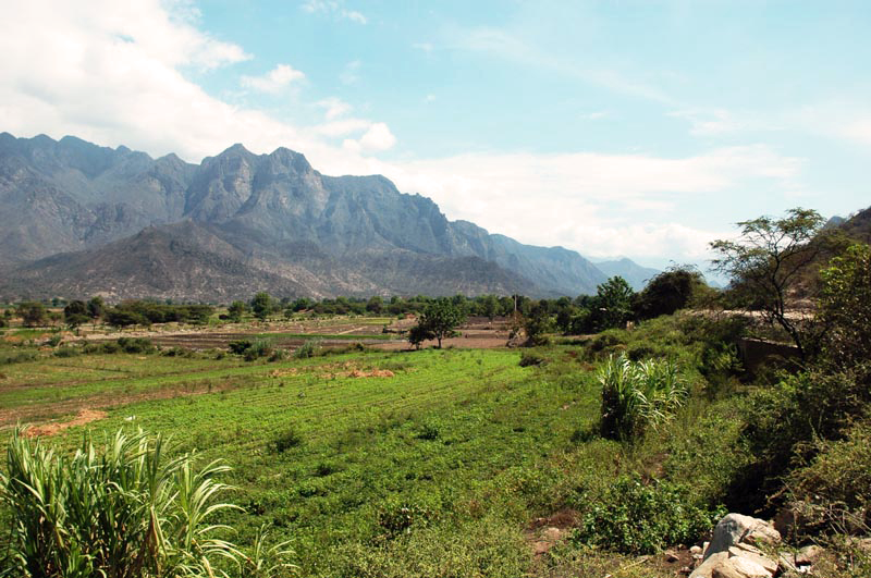
A tributary of the La Leche river, Lambayeque, Peru. WHY IS THE CASCADE OF LINEAR RESERVOIRS A METHOD OF CHOICE IN UNIT HYDROGRAPH ANALYSIS?
San Diego State University, San Diego,
California
1. INTRODUCTION
A major aim of hydrologic analysis is the
calculation of the flood hydrograph and the associated peak discharge for a given flood frequency.
For small catchments, say less than 1 square mile (2.5 km2), the peak discharge is all that may be required.
In this case, the rational method is generally the method of choice
In the decades that have elapsed since the time of its original development,
the concept of unit hydrograph has undergone major improvements in both theory and practice.
Sherman's pioneering work was followed shortly thereafter by the first synthetic unit-graph
(Snyder, 1938;
This article focuses on the cascade of linear reservoirs as a method of choice in
unit hydrograph analysis. The method is shown to have broad,
almost unlimited flexibility in simulating any and all amounts of runoff diffusion;
thus, being singularly qualified to solve the unit hydrograph and the associated composite
flood hydrograph problem.
2. MODELING CATCHMENTS/WATERSHEDS/BASINS
The modeling of surface flow in
catchments, watersheds, and basins, hereafter referred to as "basins",
is no simple matter. The objective is to convert (transform) effective rainfall into surface
runoff.
The overriding objective of surface-runoff mathematical modeling is to accurately describe the relevant physical processes of
convection
and diffusion. Convection, a first-order process, is akin to the movement of the parcels of water
in a direction parallel
to the underlying terrain. Diffusion,
Runoff diffusion is the component of surface runoff that is produced by diffusion.
The amount of diffusion was first quantified by
Hayami (1951), who combined the governing equations
of water continuity and motion, i.e., the Saint-Venant equations (Saint Venant, 1849;
in which
The unit-width discharge qo varies within a narrow range, typically less than two orders of magnitude
3. UNIT HYDROGRAPH THEORY
The rational method has no effective way
of accounting for runoff diffusion. As basins increase in surface area from small
(A < 2.5 km2) to
midsize (2.5 ≤ A < 1,000 km2), runoff diffusion becomes increasingly
important and, therefore, a more precise calculation may be required.
The larger the basin area, the more likely it is that the mean terrain slope
will be milder, although in certain unusual cases this may not be necessarily so.
To develop a way to account for runoff diffusion,
Sherman (1932) envisioned that he would typify the runoff diffusion of a given basin
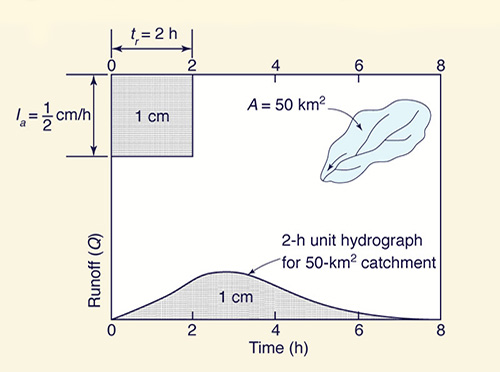
in terms of a unit hydrograph, defined as the hydrograph corresponding
to a unit depth of runoff (1 cm or 1 in) lasting "a unit increment" of time [Fig. 2 (a)].
Fig. 2 (a) The unit hydrograph.
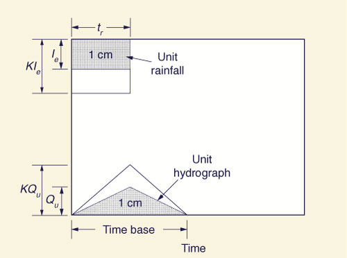
Fig. 2 (b) The unit hydrograph: Linearity.
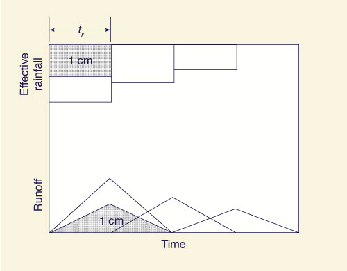
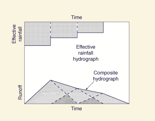
Once the unit hydrograph had been determined for a given basin, Sherman
proceeded to apply the convolution technique to calculate the composite flood
hydrograph for the corresponding effective rainfall hyetograph (the effective storm pattern).
The procedure hinges on an assumption
of linearity, that is, given a multiplier K,
the hydrograph response to rainfall amount KIe is taken as
KQe, in which
Fig. 2 (c) The unit hydrograph: Lagging.
Fig. 2 (d) The unit hydrograph: Superposition.
The unit hydrograph methodology has been used in hydrologic design for nearly 100 years.
What is sorely needed is a methodology to derive a unit hydrograph whose peak and shape are not fixed
by a certain amount of runoff diffusion specified by a formula, but one that varies with the
actual amount, be it a small or negligible amount in the case of a steep basin,
or a large or substantial
amount for a mild basin. We will show here that this variability, across the broadest range possible,
from zero (0) to infinity (∞) is clearly
provided by the method of cascade of linear reservoirs.
4. CASCADE OF LINEAR RESERVOIRS
The methodology referred to as
the cascade of linear reservoirs constitutes an effective way to simulate runoff
diffusion in a basin. As its name implies, the method is based on the connection
of several linear reservoirs in series,
wherein the outflow from the first reservoir is the inflow to the second,
the outflow from the second is the inflow to the third, and so on. Each reservoir in the series
provides a finite amount of diffusion, with the outflow from the last reservoir
reflecting the cumulative diffusion effect of all the reservoirs in the series.
Since the flow is being routed only through reservoirs, it does
not provide convection, i.e., runoff concentration (the first-order process).
However, the accumulated experience with the method has convincingly shown
that appreciable amounts of diffusion may readily be used to
model both convection and diffusion.
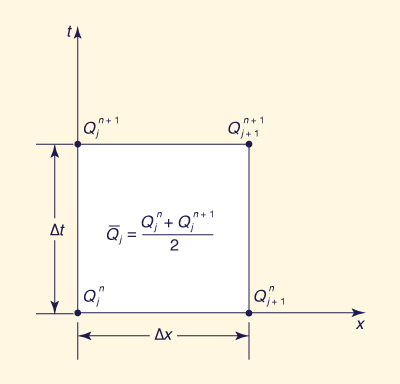
To derive the routing equation for the cascade of linear reservoirs, the point of start is the
four-point scheme (
in which Q represents discharge, whether inflow or outflow, and j and n
are spatial and temporal indices respectively (Fig. 3).
The routing coefficients C0, C1 and C2
are a function of the dimensionless ratio referred to as the Courant number
For basin routing, it is convenient to define the average inflow as follows (Fig. 3):
Substituting Eqs. 3 and Eq. 4 into Eq. 2 gives the following:
Equation 5 constitutes the routing equation of the cascade of linear reservoirs. Alternatively, through some algebraic manipulation, the following equivalent form is obtained:
Equation 6 is the routing equation of the SSARR model (U.S. Army Corps of Engineers, 1975).
Equations 5 and 6 are in a form convenient for basin routing
because the inflow is usually a rainfall hyetograph, that is, a constant average value per time interval.
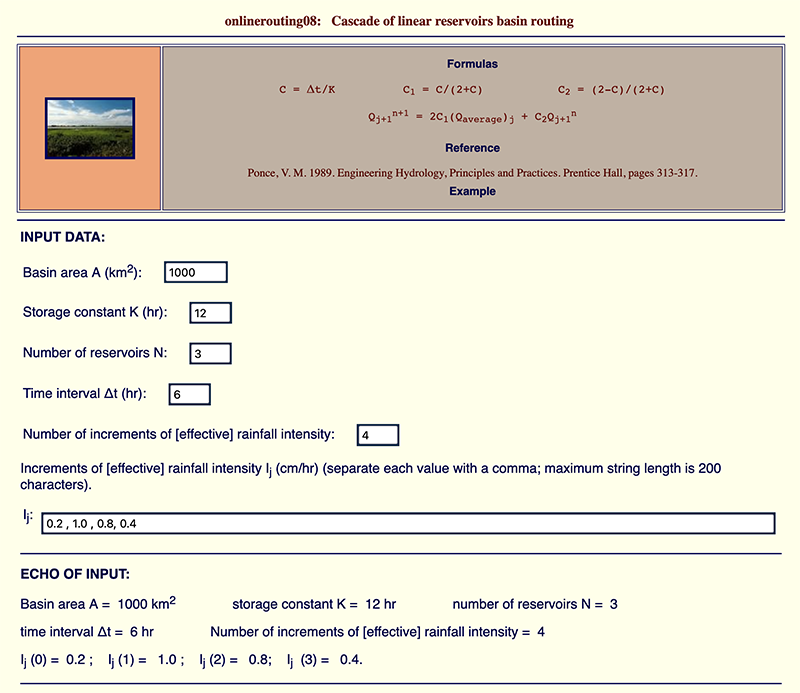
An example of a calculation by the cascade of linear reservoirs (Example 10-3) in given in
Figure 4 shows an example of the method of the cascade of linear reservoirs using the online script ONLINEROUTING08. The example reproduces the manual calculation shown in Ponce (2014a): Example 10-3, confirming the results.
5. ANALYSIS OF THE CASCADE
The cascade of linear
reservoirs (for short, CLR) calculates either: (a)
a unit hydrograph, or (b) a flood hydrograph, given the following data:
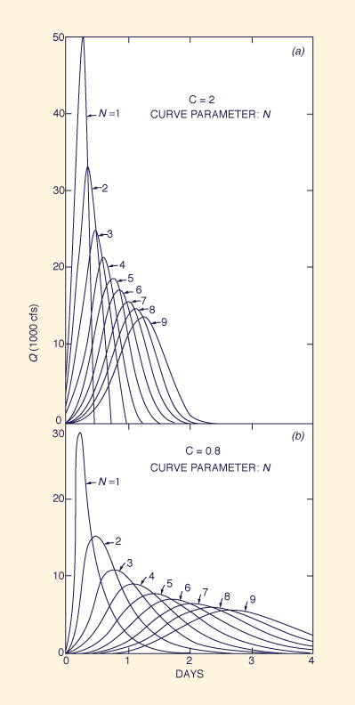
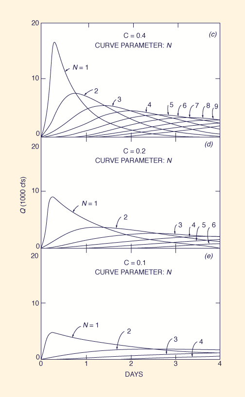
The sensitivity of the method's response to the choice of parameters
is demonstrated by the example shown in Box A
(Ponce, 1980). This example calculates a 6-hr unit hydrograph (1 inch of runoff)
for each C-N pair of a set of five (5) Courant numbers C and nine
(9) N values, for a total of forty-five (45) C-N pairs and corresponding unit hydrographs [actually, due to the great amount of
diffusion, only six (6) curves can be shown in Fig. 5 (d) and four (4) in Fig. 5 (e)].
The results are shown in Fig. 5. The maximum possible peak flow is shown to be:
Qp = 50,000 cfs
Significantly, the zero diffusion provided by the cascade
for the case of C = 2 and N = 1 results in a triangular hydrograph,
resembling that of the rational method.
For any other C-N pair,
diffusion increases with a decrease in
Courant number and an increase
in the number of reservoirs, as predicted by the theory. It should be pointed out that since C = 2 is the condition of zero diffusion, then C > 2 produces negative diffusion, that is, hydrograph amplification. In practice, diffusion requires that Δt < 2 K, i.e., the spatial interval must be smaller than twice the reservoir routing constant. Therefore, C = 2 is effectively a practical upper limit for the Courant number.
With the capability of the method of cascade of linear reservoirs amply demonstrated for generating not only
unit hydrographs (in this Section) but also composite flood hydrographs (in Section 4),
all that remains is the estimation or assessment
of the method's two routing parameters applicable to a given problem: (1) the
Courant number C, and (2) the number of reservoirs N.
6. CASCADE AND GEOMORPHOLOGY
Hayami's expression for the coefficient of hydraulic diffusivity, Eq. 1,
characterizes the behavior of runoff diffusion in basin/watershed
free-surface flow. Equation 1 reveals that diffusion is largely controlled by the
mean land surface slope. In practice, runoff diffusion manifests
itself as the attenuation of the unsteady flow features, i.e., waves and other disturbances.
The greater the mean land surface slope, the lesser the amount of diffusion, the latter
vanishing for sufficiently large slopes. By definition,
kinematic slopes, which are generally greater than 0.01 (1%),
have no diffusion.
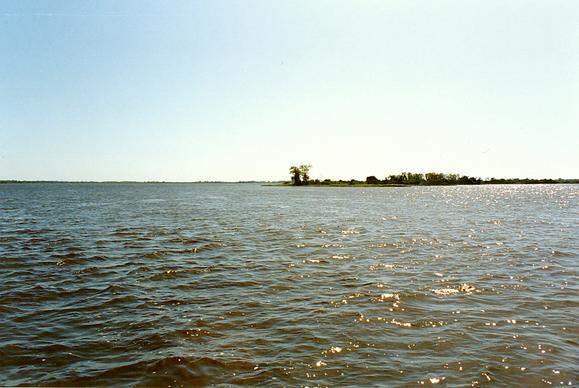
On the other side of the mean land surface slope range, for the extremely mild
values, runoff diffusion is very substantial. As mean land surface slope attains
the value of zero (i.e., a horizontal plane) diffusion becomes infinite (∞).
In this case, all waves and disturburbances
diffuse almost instantaneously, and the result is a pond or lake, arresting
surface flow [Fig. 6 (b)].
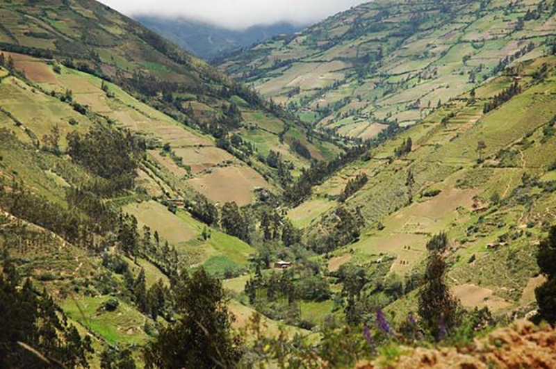
Fig. 6 (a) The Moyan watershed, headwaters
Fig. 6 (b) The Upper Paraguay river near
These observations clearly point to terrain geomorphology as the leading factor
in assessing runoff diffusion
and, consequently, in determining the shape
of the unit hydrograph and the related composite flood hydrograph.
Table 1 shows a tentative
classification of mean land surface slope, ranging from very steep (So > 0.1),
to extremely mild (So < 0.00001). The applicable cascade parameters have
been estimated by Ponce (2009b).
The peak flow Q*p
and time-to-peak t*p
of the generalized dimensionless unit hydrograph (GDUH)
have been calculated by Ponce (2009a). Note that
Q*p varies from 1 (100% of its value, kinematic flow)
for the very steep class, to 0.014 (1.4% of its value, diffusion flow)
for the
extremely mild class. Likewise,
t*p varies from 1 (1 time interval, kinematic flow)
for the very steep class, to 81
In Nature, runoff diffusion acts to obliterate the flood peaks, generally leading to milder peaks and consequently greater low flows. In extremely mild terrain geomorphology, the great amounts of diffusion lead to the occurrence of only one flood peak per year. This is the case of the Pantanal of Mato Grosso, in Brazil, where the extremely mild land slopes, close to So = 0.00001 (1 cm/km), result in only one flood peak per year in the lower basin, with its normal occurrence in May or June (Fig. 7). This fact confirms that terrain geomorphology exerts a major influence on the shape and timing of unsteady surface-water flow features.
7. ONLINE EXAMPLES
This section shows several
examples of unit hydrographs calculated by the cascade of linear reservoirs
using the online scripts developed by
Ponce (2009a).
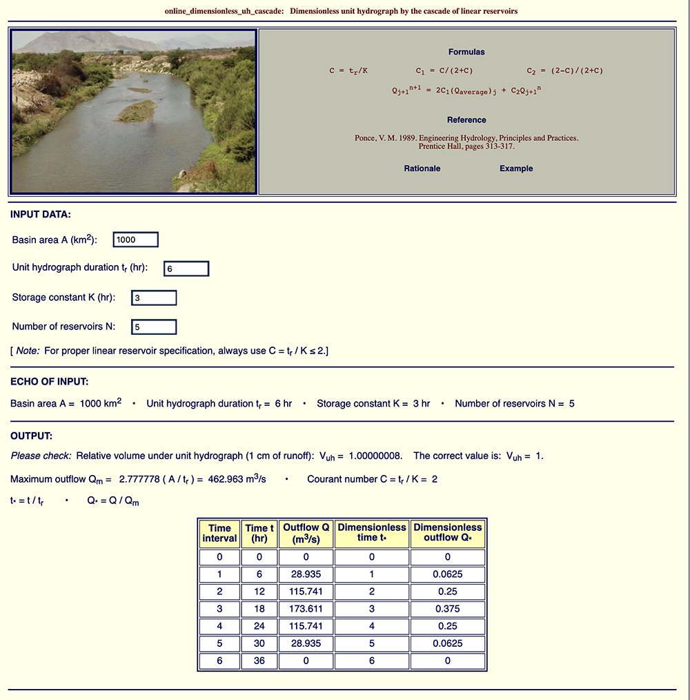
Example 1: ONLINE_DIMENSIONLESS_UH_CASCADE
Example 1A, shown in Fig. 8 (a), calculates actual and dimensionless unit hydrographs
for the following input data:
Example 1B, shown in Fig. 8 (b), uses the same basin area A and Courant number C as Example 1A,
but increases the number of reservoirs to N = 5.
The calculated peak outflow is
Examples 1A and 1B show that increasing the number of reservoirs from 3 (Example 1A)
to 5 (Example 1B)
has decreased (i.e., attenuated, diffused) the unit hydrograph peak outflow Qp from 231.482 to
Fig. 8 (a) Example 1A: Unit hydrograph
Fig. 8 (b) Example 1B: Unit hydrograph
Example 2: ONLINE_SERIES_UH_CASCADE
This example shows the calculation of dimensionless unit hydrographs for a given Courant number C and
the number of reservoirs in the range 1 ≤ N ≤ 10. For this example, C = 1. The results are shown
in Fig. 9. It is seen that diffusion increases with the number of reservoirs. For N = 1,
Q*p = 0.667
Fig. 9 Example 2: Dimensionless unit hydrographs for C = 1 and 1 ≤ N ≤ 10.
Example 3: ONLINE_ALL_SERIES_UH_CASCADE
[https://ponce.sdsu.edu/onlineallseriesuhcascade.php]
This example shows the calculation of dimensionless unit hydrographs for six (6) Courant numbers in the range
0.1 ≤ C ≤ 2.0 and ten (10) cascades
of reservoirs (N = number of reservoirs in each cascade),
with 1 ≤ N ≤ 10. The script produces sixty
Example 4: PRACTICAL APPLICATION
[https://ponce.sdsu.edu/onlinedimensionlessuhcascade.php]
Problem statement. Calculate the tr = 2-hr unit hydrograph for a basin with surface area A = 300 km2 and mean land surface slope So = 0.005.
Answer. According to Table 1, this basin is classified as mild.
Therefore, the applicable cascade parameters are estimated from this table as
We run ONLINE_DIMENSIONLESS_UH_CASCADE
with A = 300 km2,
unit hydrograph duration
The resulting dimensional and dimensionless unit hydrographs are shown in Fig. 10.
The dimensional unit hydrograph peak outflow is Qp = 36.495 m3/s at the time-to-peak tp = 22 hr.
The dimensionless unit hydrograph peak outflow is Q*p = 0.0876 at the dimensionless time-to-peak
8. SUMMARY
A review of the method of cascade of linear reservoirs for unit hydrograph development
is presented, explained, and clarified. Section 1 compares the cascade with the synthetic
unit hydrographs of Snyder and NRCS. Section 2 presents basin modeling concepts,
including Hayami's diffusivity, which characterizes
the diffusion of one-dimensional free-surface flows. Section 3 reviews concepts
of unit hydrograph theory. Section 4 explains the methodology of cascade of linear reservoirs,
deriving the routing equation and displaying actual online example calculations.
Section 5 provides an analysis of the cascade, focusing on its capability to model a broad
range of runoff diffusion effects, from zero (0) to infinity (∞). Section 6
describes the geomorphological approach to estimate the parameters of the
cascade. Section 7 provides several examples of online calculation, including
an actual practical application (Example 4).
The cascade of linear reservoirs is predicated on its capability
to model a broad
range of runoff diffusion effects, enabling increased accuracy for simulating
synthetic unit hydrographs and associated flood hydrographs. The
online computational capability enhances the method's
utility for the effective modeling
of runoff diffusion to solve a wide variety of flooding problems.
REFERENCES
Hayami, I. 1951.
On the propagation of flood waves. Bulletin, Disaster Prevention Research Institute,
No. 1, December.
Natural Resources Conservation Service (NRCS). 1985. National Engineering Handbook. Section 4: Hydrology, Washington, D.C.
(First edition: 1954).
Ponce, V. M. 1980.
Linear reservoirs and numerical diffusion.
Journal of the Hydraulics Division, Vol. 106, No. 5, May, 691-699.
Ponce, V. M. 1991.
The kinematic wave controversy.
Journal of Hydraulic Engineering, Vol. 117, No. 4, April, 511-525.
Ponce, V. M. 1995.
Hydrologic and environmental impact of the Parana-Paraguay waterway on the Pantanal of Mato Grosso, Brazil.
https://ponce.sdsu.edu/hydrologic_and_environmental_impact_of_the_parana_paraguay_waterway.html
Ponce, V. M. 2008.
La Leche river flood control project, Lambayeque, Peru.
https://ponce.sdsu.edu/0908231200.html
Ponce, V. M. 2009a.
A general dimensionless unit hydrograph.
Ponce, V. M. 2009b.
Cascade and convolution: One and the same.
Ponce, V. M., A. Taher-Shamsi and A. V. Shetty. 2003.
Dam-breach flood wave propagation using dimensionless parameters.
Journal of Hydraulic Engineering, Vol. 129, No. 10, October, 777-782.
Ponce, V. M. 2014a.
Engineering Hydrology: Principles and Practices.
Online textbook.
Ponce, V. M. 2014b.
Fundamentals of Open-channel Hydraulics.
Online textbook.
Ponce, V. M. 2023a.
When is the diffusion wave applicable?
Online paper.
Ponce, V. M. 2023b.
Kinematic and dynamic waves: The definitive statement.
Online paper.
Saint-Venant, B. de. 1871. Theorie du mouvement non-permanent des eaux avec
application aux crues des rivieres et l' introduction des varees dans leur lit, Competes Rendus
Hebdomadaires des Seances de l'Academie des Science, Paris, France, Vol. 73, 1871, 148-154.
Sherman, L. K. 1932. Streamflow from Rainfall by Unit-Graph Method.
Engineering News-Record, Vol. 108, April 7, 501-505.
Snyder, F. F. 1938. Synthetic Unit-Graphs. Transactions, American Geophysical Union. Vol. 19, 447-454.
U.S. Army Corps of Engineers. 1975.
Program Description and User Manual for SSARR Model,
Streamflow Synthesis and Reservoir Regulation. North Pacific Division,
Portland, Oregon, September, revised June, 1975.
| |||||||||||||||||||||||||||||||||||||||||||||||||||||||||||||||||||||||||||||||||||||||||||||||||||||||||||||||||||||||||||||||||||||||||||||


| 231018 |