MIXED KINEMATIC-DYNAMIC WAVES DEBUNKED
Professor Emeritus of Civil and Environmental Engineering
San Diego State University, San Diego,
California
1. INTRODUCTION
When modeling flood
waves, often the first question that comes to mind is: What type of wave should
Over the past 50 years, the approach that seems to have prevailed in some quarters is the following: "Forget
about the various types of waves; let's use
the complete solution of the St. Venant equations
in all applications, and let the computer do the number crunching!"
We note here that theory and experience have
confirmed that this approach is generally ill-fated.
Hydrodynamic theory indicates otherwise;
moreover, practical applications confirm the shortsightedness of placing all eggs in one
basket. In this article, we strive to debunk the notion that
the mixed kinematic-dynamic wave should be the only way to model flood wave propagation.
We aim to show that the sole use of the mixed wave approach is at best futile, and at worst, wrong; and
very likely to lead to wasted time and resources. For added clarity, in the following section
we list
the various types of
waves in current use, while elaborating on their nature and properties.
2. TYPES OF WAVES
In one-dimensional
unsteady free-surface flow,
the following four wave types are in general use:
3. WAVE PROPERTIES
The properties of these wave types have been examined in detail by
Ponce and Simons (1977)
Kinematic waves are those of Seddon (1900), while dynamic waves are
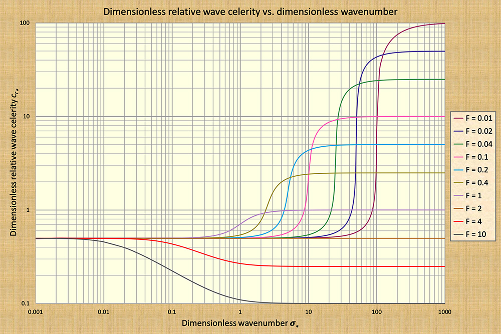
those of Lagrange (1788). Mixed kinematic-dynamic
waves are those lying along the middle-to-right of the
wavenumber spectrum (Fig. 2).
These waves, hereafter referred to as mixed waves, were featured in the numerical models
developed beginning in the 1970s to solve the complete St. Venant equations;
see, for instance, Fread (1985). These models
have been widely referred to as "dynamic wave" models,
although the misnomer has led to some confusion with the long-established Lagrange (1788) waves.
Diffusion waves
lie to the right of kinematic waves and to the left
of mixed kinematic-dynamic waves in the wavenumber spectrum (Fig. 2). Unlike kinematic waves, which feature zero diffusion,
diffusion waves have a small but perceptible amount of diffusion. However,
this diffusion is small compared to that of the mixed waves (Fig. 3).
We note that the inclusion of
Figure 2 shows that Seddon's kinematic waves,
lying toward the left of the dimensionless wavenumber spectrum,
feature a constant wave celerity and are, therefore, nondiffusive.
Following the same rationale,
Lagrange's dynamic waves, lying toward the right,
are also nondiffusive. However,
the mixed waves, lying toward the middle-to-right
and featuring sharply varying celerity,
are shown to be strongly diffusive. The amount of diffusion,
characterized by the logarithmic decrement δ, varies
with the prevailing Froude number (Fig. 3) (Wylie, 1966) (see also Box A).
Greater diffusion corresponds to the lower Froude numbers, provided the latter remains below the threshold value
4. KINEMATIC WAVES
A kinematic
wave may be indeed regarded as the quintessential flood wave.
Theory tells us that a kinematic wave does not attenuate.
Practical experience would indicate that if a wave attenuates very
quickly, it is most likely not a flood wave.
Mathematically, we reckon that the constancy of the wave celerity,
across a specified range of small dimensionless wavenumbers
(0.001 ≤ σ* ≤ 0.01),
is a sure indication of the presence of a kinematic wave
At this juncture, we endeavor to quote Lighthill and Whitham (1955), who established the foundation of kinematic wave theory. They keenly observed: "In some applications, including the case of flood waves, kinematic waves and dynamic waves are both possible together. However, the dynamic waves have a much higher wave velocity and also a rapid attenuation. Hence, although any disturbance sends some signal downstream at the ordinary wave velocity for long gravity waves [sic], this signal is too weak to be noticed at any considerable distance downstream, and the main signal arrives in the form of a kinematic wave at a much slower velocity."
5. DIFFUSION WAVES
Unlike kinematic waves,
diffusion waves are subject to a small amount of diffusion. They lie inmediately to the right of
kinematic waves in the dimensionless wavenumber spectrum,
properly within the range 0.01 ≤ σ*
≤ 0.17 (Fig. 2) (Ponce, 2024).
The value σ* = 0.01
depicts
Typical flood waves diffuse somewhat; therefore, diffusion waves are indeed a practical
model of flood wave propagation. They complement kinematic waves rather nicely, while finding their best application
in cases where
wave diffusion is appreciable and its calculation is deemed necessary.
The matter of how to best handle the numerical diffusion
has been resolved by Cunge (1969), who
proposed a match of the numerical diffusion of the scheme itself with the physical diffusion
of the related kinematic wave equation with diffusion, i.e., the diffusion wave equation.
This development led to the Muskingum-Cunge method of flood routing, a physically-based
alternative to the well-known
Muskingum method (Ponce, 2014a).
6. DYNAMIC WAVES
Classical dynamic waves are
those of Lagrange (1788). More recently, Fread (1985) and others have referred to the
mixed kinematic-dynamic waves as "dynamic" waves, while herein
we refer to them simply as "mixed" waves.
The semantic confusion is judged to be unfortunate. In an attempt to fix the problem, in this article we use the
adjective "dynamic" to refer solely to the Lagrange waves.
Dynamic waves feature
a constant wave celerity for dimensionless wavenumber
σ* ≥ 100, for most Froude numbers,
and σ* ≥ 1000 for all Froude numbers (Fig. 2).
This means conclusively, as with kinematic waves, that the dynamic waves of Lagrange are not subject to diffusion.
The dynamic waves of Lagrange are not the typical flood waves.
Their size is too small to constitute a veritable flood risk. Their appplication is restricted
to short wave propagation in irrigation and power canals, where the scale of the
disturbance is such that it may be actually seen,
or perceived, with the naked eye. Unlike flood waves, which are mass waves that feature only one wave
traveling downstream,
classical dynamic waves are energy waves, which feature two waves,
traveling in opposite directions
under subcritical flow, and in only one direction (downstream) in supercritical flow.
For enhanced clarity, a parenthetical comment regarding the cause of wave diffusion is advisable here.
Diffusion is produced by the interaction of the pressure gradient with
the friction and gravity terms (Table 1, Row 2).
More precisely defined, diffusion is produced by the interaction of the
non-kinematic (read "dynamic") terms (inertia and/or the pressure gradient), with the kinematic terms (friction
and gravity) (Table 1, Row 3) (Ponce, 1982).
7. MIXED WAVES
At this juncture, it remains for us to
discuss the only other wave type left: The mixed kinematic-dynamic wave, for short, the "mixed" wave
of unsteady open-channel flow. Since, by definition, this wave features both kinematic and dynamic
components in comparable amounts, it follows that it must be strongly diffusive.
The answer to
this question is Yes!
The mixed kinematic-dynamic wave is indeed
Within the σ*
range shown in Fig. 3, for subcritical flows (F < 1),
where the attenuation is shown to be stronger (greater values of δ), the logarithmic
decrement is seen to vary from a low of
Table 2, Line 0 (emphasized with yellow background) shows a very small amount of wave
attenuation, 0.02%, or 0.0002, associated with a very low value of logarithmic
decrement
Table 2, Line 3a (with yellow background) purposely depicts a wave attenuation of 0.3 (Col. 4), that is, a 30% decay of the
wave amplitude, a threshold value widely considered as
the division between diffusion waves (less than or equal to 30% attenuation) and
mixed waves (more than 30% attenuation) (Natural Environment Research Council, 1975).
This threshold corresponds to a value of
Table 2, Line 4a (with yellow background) purposely depicts a wave attenuation of 0.99
(Col. 4), that is, a 99% decay of the
wave amplitude, an attenuation value which nearly erases the wave altogether!
Table 2, Line 5a (with yellow background) purposely depicts a wave attenuation of 1.0
(Col. 4), that is, a 100% decay of the
wave amplitude, an attenuation value which erases the wave altogether!
This attenuation amount corresponds to a value of
Table 2, Col. 5 shows the indicated wave types, from kinematic, with very small attenuation (0.0002), to diffusion, with small to medium attenuation (0.0021 to 0.1894), to mixed wave, with large to very large attenuation (0.3 to 0.9999). Table 2, Lines 5 and 6 depict a nonexisting wave; the wave having disappeared completely, with its mass going on to form part of the underlying, or equilibrium, flow.
Given that wave attenuation is A = (1 - eδ) (Table 2, Col. 5), the results of Table 2 lead to the following waves and corresponding ranges:
We conclude that most, if not all, mixed waves would have effectively lost all their strength in most cases of practical interest. They lose their strength rapidly due to their highly diffusive nature, the latter due to the competition between kinematic and dynamic terms (read forces) that are comparable in size. It follows that mixed waves lack a basic property of a flood wave, namely, its permanency, which is characterized by its mild or very mild amount of attenuation (diffusion). Thus, we argue that, in general, mixed waves may not be construed as flood waves.
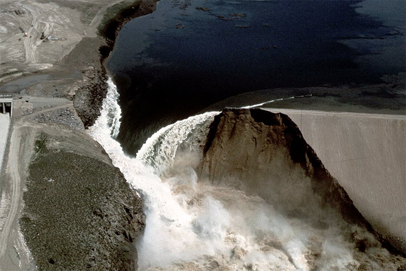
8. DAM-BREACH FLOOD WAVES
Every rule is likely to call for an exception.
In the previous section (Section 7), we presented an elaborate mathematical rationale for why the mixed wave is not likely to apply for the
case of a general flood, i.e., one that is subject to very little or no attenuation. Yet we reckon that
there is
one particular flood wave that actually may diffuse appreciably. This is the case of a dam-breach flood wave.
Typically, the flood wave produced by the breaching of an earthen embankment
is sudden, lasting about 3 hr, a sure candidate for strong wave diffusion.
A case in point:
Of 24 dam failures in the United States documented by
Such flood waves (Fig. 4) are apt to fall under the category of
mixed wave or, at the very least, be a strongly diffusive diffusion wave, with attenuation A
≅ 0.3
(see Table 2, Line 3a). Fortunately for all of us, instances of dam breaches are rare and far between.
9. MODELING FLOOD WAVES
This section elaborates on ways to model
flood waves. It seeks to answer the question: Now that I chose a type of wave, how should I proceed?
What actual tool should I use in a real practical situation? This section is divided into three parts:
(1) kinematic waves, (2) diffusion waves, and (3) mixed kinematic-dynamic waves.
The classical dynamic waves of Lagrange described in Section 6 lie outside of the scope of this section.
Kinematic waves
Kinematic wave modeling may be performed in two ways.
The first way is to realize that a true kinematic wave does not attenuate; therefore, subsidence, or
diffusion, is out of the question. Still, the wave is actually moving downstream with a certain celerity,
and that speed is subject to calculation.
Indeed, that speed is Seddon's celerity, which states
that the velocity of a flood wave at a given cross-section is equal to the slope
of the rating curve (dQ/dy) divided by the stream or channel top width (T)
(Ponce, 2014b: Eq. 10-60).
Yet an alternate way of expressing Seddon's celerity is:
c = βu, in which
The simplicity of Seddon's celerity is remarkable,
providing a ready tool to assess flood movement with a minimum of computational effort.
Box B describes an example of the application of the concept.
The second way to perform kinematic wave modeling is to use a numerical model,
many of which exist in various forms, in the literature and elsewhere. These models, however,
suffer from a decided conundrum: How to properly model a kinematic
wave without introducing a certain amount of numerical diffusion
associated itself with the finite grid size . [Note that a kinematic wave proper is not supposed to have any diffusion! See Section 4].
The diffusion in question is uncontrolled; its existence may be confirmed by running the model for
two different grid resolutions. There does not appear to be a way out of this difficulty. At this juncture, the best that can be stated is that, for a sufficiently fine grid resolution, the numerical diffusion should reduce itself to where it may not be of much concern in a given practical application. Diffusion waves Unlike kinematic waves, which are governed by a first-order differential equation, describing only convection, diffusion waves are governed by a second-order equation, describing convection and diffusion. Hayami (1951) pioneered the development of diffusion wave theory by combining the equations of water continuity and motion, excluding the inertia terms (Table 1, Line 2), into a second-order convection-diffusion equation. This methodology has been widely referred to in the literature as Hayami's diffusion analogy (Ponce, 2014a). In flood wave modeling, the numerical solution of Hayami's second-order convection-diffusion equation provides a solution of a diffusion wave. Cunge (1969) developed a convenient and practical alternative to Hayami's approach by solving the first-order kinematic wave equation numerically, while at the same time relating the amount of numerical diffusion produced by the finite grid size, to the actual physical diffusion of the second-order convection-diffusion equation of Hayami. Cunge observed that his flood routing methodology resembled the classical Muskingum method of McCarthy (1938), as cited by Chow (1959). More importantly, however, Cunge was able to tie in the numerical diffusion of the scheme itself to the physical diffusion of the flood wave in question, thus, rendering the procedure essentially grid-independent. The latter has been widely referred to as Muskingum-Cunge method (Natural Environment Research Council, 1975; Ponce and Yevjevich, 1978).
The avowed feature of grid independence does wonders to set apart the Muskingum-Cunge method from existing
kinematic wave numerical solutions,
which ostensibly suffer from grid dependence.
Mixed kinematic-dynamic waves Mixed waves comprise all terms in the
governing equations of water continuity and motion, that is, the St. Venant equations (Table, 1, Line 3).
The inclusion of the inertia terms is indeed forceful, but is not without its pitfalls.
The resulting wave
is dynamic, characteristically of second order, therefore featuring two component
waves,
which travel in different directions,
one upstream and the other downstream
in subcritical flow, and in the same direction (downstream) in supercritical flow.
Another significant pitfall is that the numerical solution of the complete St. Venant equations
represents an order-of-magnitude increase in complexity in the formulation and actual performance of the
numerical analog chosen to model the full equations. A scheme that appears to be
widely favored by practitioners is
the Preissmann box scheme (Ponce et al., 1978).
Theoretically, this scheme should provide
second-order accuracy, if only its elements (namely, the temporal and spatial derivatives)
are perfectly centered within the box, with a weighting factor θ = 0.5.
In practice, however, center-weighing the Preissmann scheme does not work,
because it leads to strong
numerical instabilities, which eventually render it inoperable.
Yet another significant pitfall of the numerical solution of the St. Venant equations is that the model does require
a downstream boundary condition to proceed. This fact was identified early by Abbott (1976): Extract, Page 276 as a decided limitation,
although later proponents of the methodology have apparently failed to pay due attention to this shortcoming.
By nature, the method generates looped rating curves at internal computational points,
forcing the need to also specify
a looped rating at the downstream boundary. Clearly, the latter requirement
is tantamount to "knowing the solution beforehand."
We point out that the comments of this subsection
purposely exclude U.S. government
software such as the U.S. Army Corps of Engineers River Analysis System,
widely known as HEC-RAS To sum up, by now it must be widely apparent that the mixed kinematic-dynamic wave is not what its users had originally in mind. The mixed wave is shown to be fraught with difficulties, the least of them being the realization of whether the said wave is there or not for us to calculate it! More commonly, the modeler will face other problems, of both a numerical and physical nature, which will have the net effect of casting doubts on the accuracy and practicality of the overall procedure.
10. ANALYSIS AND CONCLUSIONS
We have analyzed the celerity and attenuation
properties of four types of shallow-water waves currently in use in hydraulic engineering:
(1) kinematic, (2) diffusion, (3) mixed kinematic-dynamic, and
We have sought to answer the question of whether the mixed wave is generally too strongly diffusive
to be considered a practical flood wave. The answer is Yes! In the great majority of cases,
the mixed waves may not be there for us to calculate them!
Their typical midsize obliges them to attenuate very quickly, with their
mass eventually joining the underlying kinematic or diffusion wave,
which continues to grow in both size
and permanence as it propagates downstream.
Note that only in the extremely unusual case of a dam-breach flood wave could
we be actually confronted with the case of a mixed flood wave.
A dam-breach flood wave is characteristically sudden, poised by Nature to be a mixed wave, an unusual type of flood wave [The experience of the
Teton dam failure (Fig. 4) is a case in point].
Professionals in charge of forecasting or hindcasting a dam-breach flood wave would be keen to keep this in mind.
For all other flood wave routing applications, the kinematic and diffusion waves should do the job in an accurate and
forthright manner.
Notably, since a diffusion wave will actually calculate diffusion, including the case of zero diffusion,
it follows that the solution of a diffusion wave encompasses the solution of a kinematic wave.
Therefore, the diffusion wave is postulated as the flood wave par excellence, i.e., the type of wave generally indicated for
use in practical applications
of flood routing, analysis, and design.
11. CLOSING REMARKS
In general, mixed kinematic-dynamic waves,
herein simply referred to as mixed waves,
and which elsewhere have been widely referred to, albeit inaccurately,
as "dynamic waves," are in fact not
large enough nor permanent enough to veritably constitute flood waves.
An accumulated body of
theory and experience confirms this fact.
On the other hand, kinematic waves
and their close cousins, diffusion waves,
typically feature large mass and are characteristically nondiffusive, i.e.,
either they are not attenuating or, else,
attenuating only a very small amount; therefore,
they are apt to be ideal models of flood waves.
Since a numerical solution of a diffusion wave generally
comprises that of a kinematic wave,
the diffusion wave may be regarded as the most appropriate way to model
flood waves.
REFERENCES
Abbott, M. B. 1976. Computational hydraulics: A short pathology: Extract: Page 276. Journal of Hydraulic Research, Vol. 14, No. 4, 271-285.
Chow, V. T. 1959. Open-channel hydraulics. McGraw-Hill, New York, NY.
Cunge, J. A. 1969. On the
Subject of a Flood Propagation Computation Method (Muskingum Method).
Journal of Hydraulic Research, 7(2), 205-230.
Fread, D. L. 1985. "Channel Routing," in Hydrological Forecasting,
M. G. Anderson and T. P. Burt, eds., Wiley, New York.
Hayami, I. 1951.
On the propagation of flood waves. Bulletin, Disaster Prevention Research Institute,
No. 1, December.
HEC-RAS. Hydrologic Engineering Center River Analysis System,
U.S. Army Corps of Engineers, Davis, California. Wikipedia citation (consulted
May 15, 2024).
Lagrange, J. L. de. 1788. Mécanique analytique, Paris, part 2, section II, article 2, 192.
Lighthill, M. J. and G. B. Whitham. 1955.
On kinematic waves. I. Flood movement in long rivers.
Proceedings,
McCarthy, G.T. 1938. "The Unit Hydrograph and Flood Routing,"
unpublished manuscript, presented at a Conference of the North Atlantic Division,
U.S. Army Corps of Engineers, June 24.
(Cited by V. T, Chow's text "Open-channel Hydraulics," page 607).
Natural Environment Research Council. 1975. Flood Studies Report,
Vol. III: Flood Routing Studies, London, England.
Ponce, V. M. and D. B. Simons. 1977.
Shallow wave propagation in open channel flow.
Journal of Hydraulic Engineering, ASCE, 103(12), 1461-1476.
Ponce, V. M. and V. Yevjevich. 1978.
Muskingum-Cunge Method with Variable Parameters.
Journal of the Hydraulics Division, ASCE, 104(12), December, 1663-1667.
Ponce, V. M., H. Indlekofer, and D. B. Simons. 1978.
Convergence of four-point implicit water wave models.
Journal of the Hydraulics Division, ASCE, 104(7), July, 947-958.
Ponce, V. M. 1982.
Nature of wave
attenuation in open-channel flow. Journal of Hydraulic Engineering, ASCE, 108(HY12), February, 257-262.
Ponce, V. M. and D. Windingland. 1985.
Kinematic shock:
Sensitivity analysis. Journal of Hydraulic Engineering, ASCE, 111(4), April, 600-611.
Ponce, V. M. 1986.
Diffusion wave modeling of catchment dynamics.
Journal of Hydraulic Engineering, 112(8), August, 716-727.
Ponce, V. M. 1995.
Hydrologic and environmental impact of the Parana-Paraguay waterway on the Pantanal of Mato Grosso, Brazil.
https://ponce.sdsu.edu/hydrologic_and_environmental_impact_of_the_parana_paraguay_waterway.html
Ponce, V. M. 2014a.
Engineering Hydrology: Principles and Practices.
Online textbook.
Ponce, V. M. 2014b.
Fundamentals of Open-channel Hydraulics.
Online textbook.
Ponce, V. M. 2024.
Kinematic waves demystified. Online publication.
Seddon, J. A. 1900. River Hydraulics. Transactions, American Society of Civil Engineers, Vol. XLIII, 179-243, June; Extract: pages 218-223.
Taher-Shamsi, A., A. V. Shetty, and V. M. Ponce. 2003.
Embankment dam breaching: Geometry and peak outflow characteristics.
Online report.
Wylie, C. R. 1966. Advanced Engineering Mathematics, 3rd ed., McGraw-Hill Book Co., New York, NY.
| |||||||||||||||||||||||||||||||||||||||||||||||||||||||||||||||||||||||||||||||||||||||||||||||||||||||||||||||||||||||||||||||||||||||||||||||||||||||